Quantization Explained: How to Run AI Models with Less Memory

Quantization Explained: How to Run AI Models with Less Memory

Try to load Llama 3.1 70B on your own hardware in its native precision and you hit a wall fast: roughly 140GB of memory just to hold the weights, before you’ve generated a single token. Most people don’t have that, and neither do most companies running a lean inference budget.

The same wall shows up at smaller scale too. A 13B model that runs fine on a high-end workstation refuses to fit on a laptop, and a cloud GPU bill for serving a chatbot in full precision can be two or three times higher than it needs to be.

Quantization is the technique that gets you out of that wall. Understanding how it actually works — not just that it “makes models smaller” — is what lets you use it without quietly wrecking your model’s accuracy.

Quantization is the process of representing a model’s weights, and sometimes its activations, using fewer bits of numerical precision than the format the model was trained in. Cutting a model from 16-bit precision down to 4-bit precision shrinks its memory footprint by roughly 75%.

For most practical bit-widths, that reduction comes with a measurable but modest quality cost rather than a catastrophic one. The rest of this guide explains the mechanism behind that trade-off, shows exactly how much memory different model sizes actually need, and walks through real, cited quality-loss data so you’re not guessing at how much accuracy you’re giving up.

This article owns the mechanism: why quantization works at all, why it sometimes breaks, how much memory a given model actually needs once you do the arithmetic yourself, and which method fits which real-world constraint. It deliberately does not try to be a click-by-click tutorial for every tool and operating system combination.

That level of hands-on walkthrough belongs to a dedicated companion piece on running models locally, later in this series. Think of this as the article that tells you what’s actually happening and what to choose; the practical step-by-step comes next.

What “Precision” Actually Means for a Model

A model’s precision determines how many bits it spends representing each of its weights — and that choice trades accuracy for memory in a direct, measurable way.

Every weight inside a neural network — including the large language models covered in our guide to what a large language model actually is — is just a number. During training, those numbers are almost always stored and updated in 32-bit floating point (FP32) or, more commonly today, 16-bit formats like FP16 or BF16.

The bit width determines how many distinct values a number can represent and how much decimal precision it carries. FP32 gives roughly seven meaningful decimal digits of precision; FP16 and BF16 cut that to about three, trading precision for half the memory and faster computation.

Quantization pushes this further, down to 8-bit integers (INT8), 4-bit integers (INT4), or even lower. The complication is that neural network weights are continuous, often small, and distributed roughly like a bell curve — they don’t map cleanly onto a small set of integers the way pixel values in an 8-bit image do.

So quantization has to build a mapping between the real-valued weights and a limited set of integer buckets, then remember how to convert back. The standard version is called affine or linear quantization: a scale factor and a zero-point are calculated from the range of the weights being compressed.

Each real value is divided by the scale and rounded to the nearest integer. At inference time the process runs in reverse, multiplying the stored integer back by the scale to recover an approximation of the original value.

The weight you get back is never exactly the one you started with. It’s the closest value the chosen bit-width can represent, and that rounding error is the entire cost of quantization.

A quick worked example makes this concrete. Say a layer’s weights peak at 0.8 in magnitude, and you’re quantizing to symmetric INT8, which offers 127 positive integer steps. The scale factor is 0.8 divided by 127, or roughly 0.0063.

A weight of 0.35 divides by that scale to about 55.6, rounds to the integer 56, and gets stored as 56 instead of 0.35. Dequantizing multiplies back: 56 × 0.0063 ≈ 0.353 — close to the original value, off by about 0.003.

That small, per-weight error, repeated across billions of weights in a layer, is the entire mechanism the rest of this guide is about controlling.

What makes this workable at all, rather than a strategy that quietly destroys every model it touches, is that neural networks are heavily over-parameterized. A model with billions of parameters has enormous redundancy in how it represents what it has learned, so a small, evenly distributed rounding error on each individual weight tends to average out across a layer rather than compound into a large output error.

That’s the actual mechanism behind “quantization doesn’t hurt accuracy that much.” It isn’t magic — it’s the same statistical robustness that lets these models tolerate dropout, noise injection, and other training-time perturbations without falling apart.

Why Naive Quantization Breaks at Scale

Quantization stops being simple past a certain model size, because large models develop extreme value outliers that a basic rounding scheme handles badly.

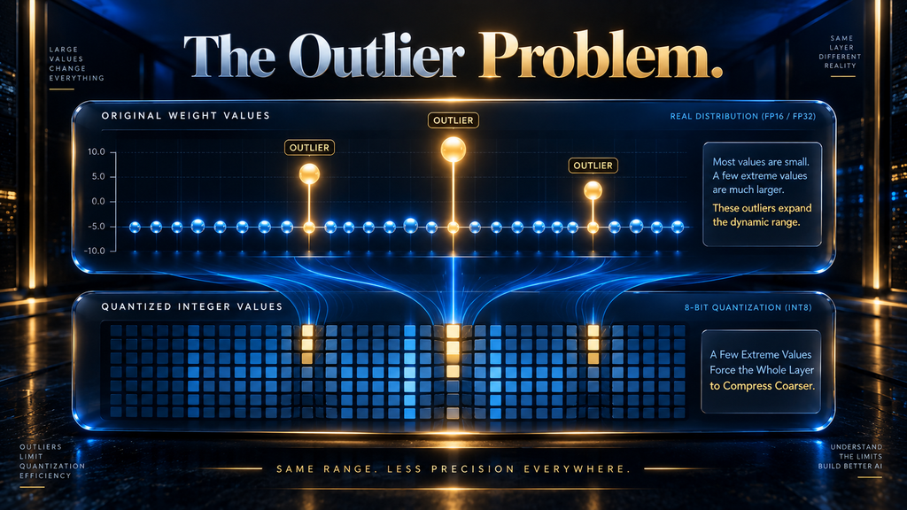
Once transformer language models cross roughly 6.7 billion parameters, certain activation channels — not weights, activations, the intermediate values flowing through the network during a forward pass — start developing extreme outlier values concentrated in a small number of feature dimensions. This was documented directly by Tim Dettmers and coauthors in the LLM.int8() paper.

Their research showed that naive uniform 8-bit quantization applied across an entire layer, outliers included, causes a sharp and sometimes catastrophic drop in model quality specifically at this scale — even though the same naive approach works fine on smaller models. The problem is that a linear quantization scheme sets its scale factor based on the full range of values it needs to represent.

A handful of extreme outliers stretch that range enormously, which forces every other, ordinary-magnitude value in that same layer to be compressed far more coarsely than it would be otherwise. That single finding is why quantization isn’t one technique with several interchangeable names — it’s a family of genuinely different approaches, each built to solve the outlier problem in a different way.

LLM.int8() itself solves it by decomposition: it identifies where outliers concentrate, keeps just those dimensions in FP16, and quantizes everything else to INT8, recombining the two at computation time. A related technique called SmoothQuant takes a different angle: it multiplies each troublesome activation channel by a small factor before quantizing it, and divides the corresponding weight channel by that same factor afterward.

That rescaling is mathematically equivalent, so the layer’s output is unchanged, but it shifts the burden of representing a wide numeric range away from activations — which are hard to calibrate ahead of time because they depend on the input — and onto weights, which are fixed and far easier to quantize accurately.

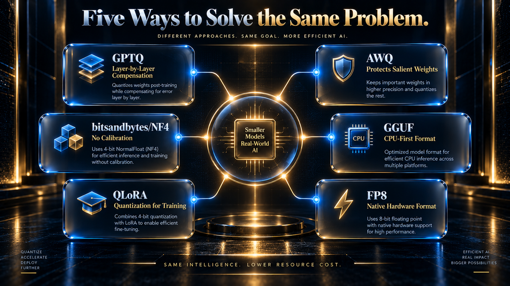
GPTQ and AWQ, the two methods most commonly used for serious 4-bit compression today, solve the same underlying problem through entirely different logic. Understanding that difference is the difference between picking a quantization method by vibes and picking one that actually fits your model and hardware.

The Major Quantization Methods, and How They Actually Differ

GPTQ: Calibrated, Layer-by-Layer Compensation

GPTQ compensates for rounding error one layer at a time, using a small calibration dataset to decide the safest order to round weights in.

GPTQ, introduced by Frantar, Ashkboos, Hoefler, and Alistarh in their 2023 paper, doesn’t try to protect outlier values directly. Instead, it quantizes a model layer by layer, using second-order curvature information — an approximation of the Hessian, built from a small calibration dataset run through the model — to decide the order in which weights get rounded.

It also adjusts the weights that haven’t been quantized yet to compensate for the error just introduced. In effect, every rounding decision in a layer is made aware of the decisions that came before it, so errors are actively corrected against rather than allowed to accumulate independently.

This calibration step is also GPTQ’s main practical dependency. The quality of the compensation depends on how representative the calibration data is of what the model will actually see in production.

The original paper’s own experiments used just 128 random 2,048-token segments pulled from the C4 dataset — generic crawled web text, not task-specific data. The authors describe this deliberately as a “zero-shot” setup: GPTQ never sees examples of the task it will actually be used for, which is precisely why calibrating on your own domain data instead of accepting a generic default can measurably change the result.

A model calibrated on generic web text and then deployed on legal or medical documents can come out measurably worse on that specific domain than the published benchmark numbers would suggest. The data you calibrate or train on has to resemble the data you’ll actually run against, or the numbers you validated against don’t transfer.

That’s the same lesson covered in more depth in our guide to preparing a dataset for fine-tuning.

AWQ: Protecting the Weights That Actually Matter

AWQ skips per-weight compensation entirely and instead protects the small fraction of weights that the model’s own activations reveal as most important.

AWQ, introduced by Lin and coauthors and awarded Best Paper at MLSys 2024, starts from a different observation: not every weight in a layer matters equally to the final output. The weights that matter most — the “salient” ones — can be identified not by their own magnitude, but by the magnitude of the activations they get multiplied against.

A weight connected to a small, unimportant activation can be compressed aggressively with little consequence. A weight connected to a large, important activation causes outsized error if compressed the same way.

Rather than solving this per-weight the way GPTQ does, AWQ computes a per-channel scaling factor that protects roughly the top 1% of salient weight channels, at a small, deliberate cost to the rest. Because this approach doesn’t require reconstructing and compensating an entire layer’s weights sequentially, AWQ models often decode faster at inference time than GPTQ models of equivalent bit-width.

In hands-on benchmark testing published by Cast.ai, a quantized Mistral 7B model ran inference in 4.96 seconds under AWQ versus 8.78 seconds under GPTQ on the same A100 GPU. That gap was driven by dequantization overhead, not by any difference in model quality between the two.

bitsandbytes and NF4: The No-Calibration GPU Baseline

bitsandbytes trades some inference speed for the simplest possible setup: no calibration dataset, no conversion step, just a flag in your load call.

The bitsandbytes library, built on the LLM.int8() work described above, offers the lowest-friction path to quantization inside the Hugging Face ecosystem. Loading a model with load_in_8bit=True or load_in_4bit=True quantizes it on the fly, with no calibration dataset and no separate conversion step.

Its 4-bit mode introduced a genuinely useful innovation in the QLoRA paper by Dettmers, Pagnoni, Holtzman, and Zettlemoyer: a data type called NF4 (NormalFloat4), which is quantile-based rather than linear. Neural network weights cluster around zero in roughly a bell-curve distribution.

Allocating the 16 available 4-bit buckets according to that distribution — more buckets near the center, fewer at the tails — represents the actual weight distribution more faithfully than evenly spaced linear buckets would.

The trade-off is that on-the-fly quantization, while convenient, is generally not the fastest option at inference time. It still carries some of the mixed-precision overhead needed to handle the outlier problem described earlier.

GGUF: A File Format, Not an Algorithm

GGUF is a container, not a compression method — the actual quantization happens through the k-quant and i-quant schemes packed inside it.

GGUF is the format used by llama.cpp and its ecosystem, and it’s worth being precise about what it actually is, because it’s commonly misdescribed: GGUF is a container file format, not a quantization algorithm in its own right. The actual compression schemes packed inside a .gguf file are the “k-quants” (named things like Q4_K_M, Q5_K_M, Q6_K) and newer “i-quants” for more extreme compression.

According to the official llama.cpp quantization documentation, applied to Llama 3.1 8B, Q4_K_M uses about 4.89 bits per weight and produces a 4.58 GiB file. Q5_K_M uses about 5.70 bits per weight at 5.33 GiB, Q6_K uses about 6.56 bits per weight at 6.14 GiB, and Q8_0 uses about 8.50 bits per weight at 7.95 GiB, against a 14.96 GiB FP16 baseline for the same model.

GGUF’s real advantage isn’t a smarter compression algorithm than GPTQ or AWQ. It’s first-class CPU inference support and the broadest hardware compatibility of any current quantization ecosystem, which is why it’s the default choice for running models on a laptop or a machine with no dedicated GPU.

QLoRA: Quantization for Fine-Tuning, Not Just Inference

QLoRA uses quantization for a different purpose than every method above: making a model affordable to train, not just to run.

Every method above compresses a model so it can run more cheaply. QLoRA, from the same Dettmers paper that introduced NF4, does something different: it makes it possible to fine-tune a model you couldn’t otherwise afford to touch.

The base model is frozen in 4-bit NF4 precision, and only a small set of newly added LoRA adapter matrices train in higher precision on top of it. QLoRA adds two more tricks: double quantization, which compresses the quantization constants themselves, and paged optimizers, which absorb memory spikes using CPU memory as overflow.

The practical result, demonstrated in the original paper, is that a 65-billion-parameter model can be fine-tuned on a single 48GB GPU with no measurable loss in output quality compared to full 16-bit fine-tuning. That’s a workload that would otherwise require multiple high-end GPUs running in parallel.

This is also the method that ties quantization directly back into fine-tuning a model at all. If your goal is training, not just serving, QLoRA is usually the entry point, not the inference-focused methods above.

FP8: The Native Hardware Format

FP8 solves the outlier problem differently from every method above simply by staying a floating-point format instead of becoming an integer one.

The methods above all quantize into integer formats, which need an explicit scale-and-zero-point mapping to represent real numbers. FP8 takes a different path: it’s still a floating-point format, just an 8-bit one, which means it keeps a wider dynamic range than an 8-bit integer at the cost of less precision within that range.

That makes it naturally more resilient to the outlier problem described earlier, since floating point formats represent very small and very large numbers without a separate correction scheme. NVIDIA’s Hopper and Blackwell GPUs include native FP8 support through the Transformer Engine.

FP8 isn’t a drop-in replacement for GPTQ or GGUF on consumer hardware, since it needs that specific hardware support to deliver a real speed benefit. On the GPUs that support it, though, it’s becoming the default rather than a specialized option.

The AHW Quantization Memory Calculator: How Much Memory Do You Actually Need?

The exact memory a model needs is simple arithmetic once you know the formula — most explainers skip giving you the numbers to apply it yourself.

Most quantization explainers describe the trade-off in the abstract without giving readers the arithmetic to apply it to their own situation. The relationship is straightforward: memory in gigabytes is approximately equal to the number of parameters, in billions, multiplied by the bytes used per parameter at a given precision — 4 bytes for FP32, 2 bytes for FP16 or BF16, 1 byte for INT8, and 0.5 bytes for INT4.

The table below applies that arithmetic across the model sizes you’re most likely to actually encounter.

Model size	FP32 (4 bytes)	FP16/BF16 (2 bytes)	INT8 (1 byte)	INT4 (0.5 bytes)
3B	12 GB	6 GB	3 GB	1.5 GB
7B	28 GB	14 GB	7 GB	3.5 GB
13B	52 GB	26 GB	13 GB	6.5 GB
34B	136 GB	68 GB	34 GB	17 GB
70B	280 GB	140 GB	70 GB	35 GB
405B	1,620 GB	810 GB	405 GB	202.5 GB

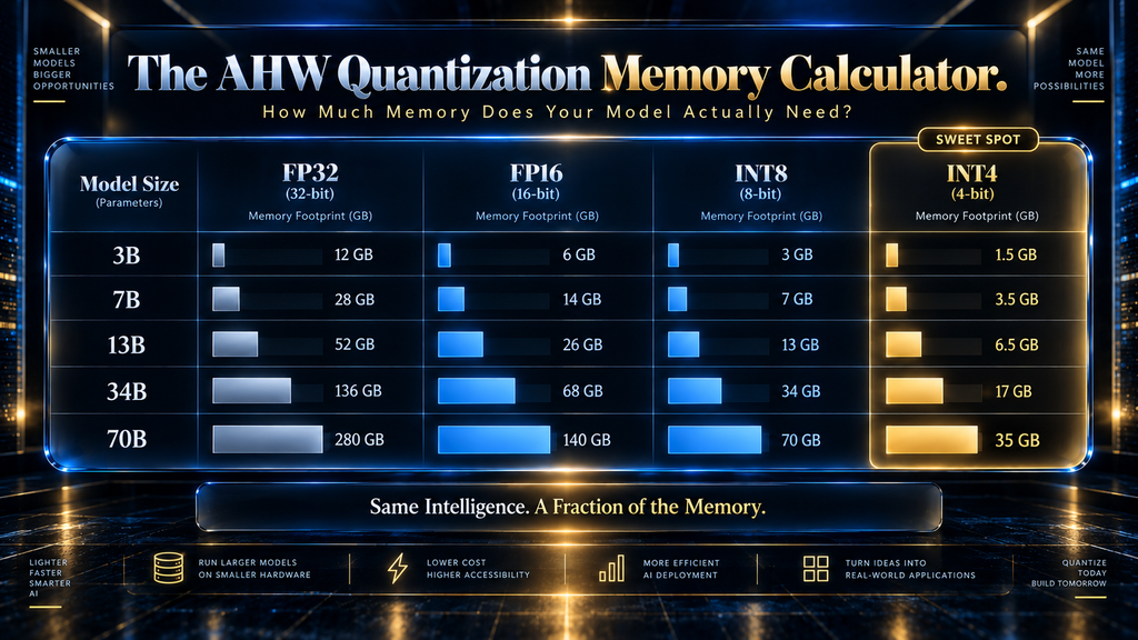
This table is weights-only, and it’s important not to treat it as your complete memory budget. Running inference also requires memory for the KV cache, which grows with both context length and batch size, plus activation memory during the forward pass itself.

For a long-context, high-batch-size deployment, that overhead can add a meaningful amount on top of the weight footprint shown here. Treat these numbers as the floor, not the total.

What the table does make concrete is the scale of the actual decision. Moving a 70B model from FP16 to INT4 is the difference between needing 140GB, out of reach on almost any single consumer setup, and needing 35GB, which fits on a single high-end GPU or a well-specced workstation.

From Memory Savings to Dollar Savings

The memory table above isn’t just an academic exercise — it directly determines which GPU tier you can rent, and GPU tiers don’t scale linearly in price. As of late 2026, dedicated-cloud A100 80GB instances run roughly $2.21–$2.70 per hour, and H100 80GB instances run $1.99–$3.99 per hour, according to pricing tracked by CloudZero.

L4 24GB instances, by contrast, run closer to $0.44–$0.80 per hour on the same tracker — under a third of the cost. A 70B model that needs INT4 quantization to drop from 140GB down to 35GB doesn’t just become runnable on cheaper hardware; it can move an entire deployment out of the most expensive GPU tier and into a materially less expensive one.

This has a second-order effect beyond the sticker price of the instance itself. A smaller memory footprint per model leaves more headroom on the same card for larger batch sizes or additional concurrent requests, so the same GPU can serve more simultaneous users without adding hardware. For anyone serving a model in production rather than running it locally for personal use, quantization is as much a cost-engineering decision as a technical one.

How Much Quality Do You Actually Lose?

Real, cited data shows the quality cost of quantization is small down to about 4-bit, then rises sharply below it — this is the question every practical quantization decision comes down to, and it’s the one most explainers answer with a vague gesture at “some accuracy loss” rather than real numbers.

A January 2026 evaluation, “Which Quantization Should I Use? A Unified Evaluation of llama.cpp Quantization on Llama-3.1-8B-Instruct,” measured exactly this across the k-quant family, using perplexity and a composite of downstream benchmarks spanning reasoning, knowledge, instruction-following, and truthfulness.

Against an FP16 baseline perplexity of 7.32, Q8_0 scored 7.33, Q6_K scored 7.35, Q5_0 scored 7.43, and Q4_K_M scored 7.56 — each step down in precision costing a small, gradually increasing amount. The picture changes sharply below that: Q3_K_S scored 8.96, a much larger jump than the gap between any of the 4-bit-and-above levels.

The same pattern held on the composite benchmark score. Q4_K_S lost only 0.43 percentage points relative to the FP16 baseline’s 69.47%, while Q3_K_S lost 5.73 percentage points — more than thirteen times the degradation for a roughly comparable additional step down in precision.

The practical takeaway isn’t just “lower precision costs more accuracy,” which is obvious. It’s that the cost curve has a distinct knee, not a smooth slope.

From FP16 down through roughly the 4-bit range, quality degrades gently and close to linearly with the size savings you’re getting. Below that, in the 3-bit and 2-bit range, degradation accelerates disproportionately relative to the additional compression gained — you give up file size at a worsening exchange rate the further down you push.

This is consistent with the broader body of quantization research: the original GPTQ paper reported similarly modest perplexity increases when compressing OPT and BLOOM family models to 4-bit. That corroborates that the “4-bit is close to free, below that gets expensive” pattern isn’t specific to one paper or one model family.

For most production use cases, this is the reason 4-bit-class quantization — GPTQ, AWQ, or Q4_K_M/Q5_K_M in the GGUF family — has become the default rather than the exception. Going further usually needs a specific, deliberate reason rather than being the default choice for “more compression is always better.”

How to Evaluate a Quantized Model Before You Ship It

The published numbers above are for one specific model, so validating your own before deploying is a short but necessary extra step.

The numbers above are for Llama-3.1-8B-Instruct specifically, and they will not transfer exactly to a different model family, size, or task. Before deploying any quantized model, run the same basic checks yourself rather than assuming published numbers apply.

Compare perplexity on a sample of your own domain text, not just a generic benchmark corpus — a model can look fine on Wikipedia-style text and still degrade on your specific content. Run a small, fixed set of real prompts from your actual use case through both the full-precision and quantized versions side by side, and compare the outputs directly rather than relying on a single aggregate score.

For task-specific deployments, add a narrow benchmark that matches what the model will actually do — a set of classification examples, instruction-following prompts, or a small held-out evaluation set from your own data. The general reasoning and knowledge benchmarks cited above won’t necessarily catch a regression specific to your task.

This is a short process, usually a few hours of testing. It’s the difference between finding out a quantization level doesn’t work for you before it ships, rather than after.

Where Quantization Actually Breaks

Quantization is reliable within its tested range, but three specific failure patterns show up once you push past the conditions it was validated under.

Extreme low-bit compression, at 2-bit and in the more aggressive 3-bit variants, degrades disproportionately on tasks that require multi-step reasoning or precise instruction-following. This happens even when the aggregate perplexity number looks only moderately worse — a model can retain fluent, grammatical output while losing the reliability of its actual reasoning chain, which perplexity alone doesn’t fully capture.

Calibration-dependent methods like GPTQ and AWQ inherit whatever gap exists between the calibration data and your real deployment data. A quantized model validated against a general benchmark can underperform specifically on a specialized domain if the calibration set didn’t represent that domain, which is a data problem more than an algorithm problem.

There’s also a hardware trap that catches people who assume file size and inference speed are the same thing. Not every quantization format has an optimized compute kernel on every GPU or CPU architecture, and a smaller file running on hardware without a fast kernel for that format can end up slower than a larger, better-supported one.

Checking kernel support for your hardware before committing to a format matters as much as checking file size. And stacking quantization on quantization — re-compressing an already-quantized model, or fine-tuning on top of one without an adapter-based approach — compounds rounding error in ways that don’t scale linearly.

That compounding risk is part of why QLoRA freezes the quantized base model rather than continuing to update its quantized weights during training.

Quantization and Fine-Tuning: What Happens When You Combine Them

Quantization and fine-tuning intersect in one specific way — QLoRA — and the order you apply them in is what makes it work.

The relationship between quantization and fine-tuning runs in both directions, and it’s worth being explicit about which direction you actually need. If your goal is to run an already-trained model more cheaply, you quantize after training is done, using GPTQ, AWQ, or GGUF as covered above — fine-tuning doesn’t enter into it.

If your goal is to train or adapt a model you couldn’t otherwise afford to fine-tune at full precision, QLoRA is the tool, and the order matters. Quantize the frozen base model first, then train small adapters on top of it, rather than trying to fine-tune a model that’s already been quantized for inference and wasn’t set up for training.

The data quality principle carries over regardless of which direction you’re working in. A GPTQ or AWQ calibration set that doesn’t represent your deployment domain produces a quantized model that underperforms on exactly the cases you care about, in the same way a training dataset that doesn’t represent your target task produces a fine-tuned model that underperforms on it.

The specific mechanics covered in our dataset preparation guide apply just as directly to a calibration set as to a fine-tuning set, even though the two serve different technical purposes. Neither quantization nor fine-tuning is a substitute for representative data — they’re both downstream of it.

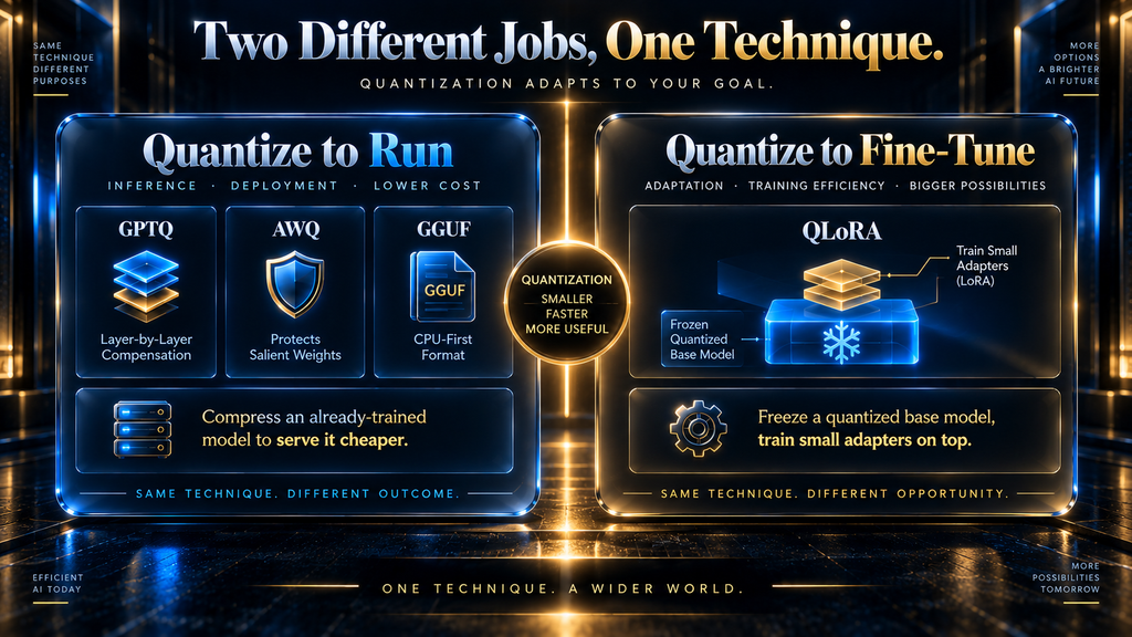
The AHW Quantization Decision Framework

The right quantization method depends entirely on your hardware and your goal, not on which name is currently trending — this table sorts by scenario, not by tool.

Most of the guidance available online tells you what GPTQ, AWQ, and GGUF are without telling you which one actually fits your situation. The table below is built directly from the mechanism and evidence covered above, organized around the constraint you’re actually working with.

Your situation	Recommended approach	Why
Running a model locally with no dedicated GPU	GGUF, Q4_K_M or Q5_K_M	Best CPU kernel support of any format; Q4_K_M/Q5_K_M sit above the quality “knee” described earlier
Running a model on a consumer GPU (8–24GB VRAM)	GGUF or GPTQ, 4-bit	Fits comfortably per the memory table above; GPTQ has broad tooling support if GPU-only
Serving a model at scale, latency-sensitive	AWQ, or FP8 on Hopper/Blackwell hardware	Faster dequantization than GPTQ at equivalent bit-width; FP8 gets native hardware acceleration where available
Fine-tuning a large base model on limited GPU memory	QLoRA (4-bit NF4 + LoRA adapters)	Makes fine-tuning models otherwise out of reach feasible on a single GPU, per the QLoRA paper’s own 65B-on-48GB result
Maximum compression for edge or mobile deployment	GGUF, Q3_K or IQ-series, with explicit quality testing	Accept the steeper degradation below 4-bit only when the deployment constraint genuinely requires it
Near-lossless compression, moderate savings acceptable	Q6_K/Q8_0 or 8-bit bitsandbytes	Perplexity essentially matches FP16 per the cited 2026 evaluation, while still cutting memory meaningfully

Notice that the table above never says a single format is “best” — it always ties the recommendation to what you’re actually trying to do. A format that’s the right choice for CPU-only local inference is a poor choice for a latency-sensitive GPU serving deployment, and neither has anything to do with which one you’d pick for fine-tuning rather than inference.

The table also assumes you have some choice of hardware, and for many readers that isn’t quite true. According to Hugging Face’s own quantization method matrix, GGUF and its Metal backend have first-class support on Apple Silicon, while AWQ and several other methods extend to AMD’s ROCm stack.

If you’re on a Mac rather than a Windows or Linux machine with an NVIDIA card, GGUF is usually the realistic default regardless of which method the table above would otherwise point you toward — the hardware layer narrows your options before the use-case layer does.

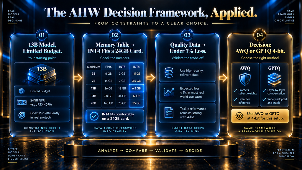
Putting It Together: A Worked Scenario

Take a team trying to serve a 13B customer-support model to real users on a limited infrastructure budget. The memory table earlier in this guide already rules out FP16, which needs 26GB and won’t fit comfortably on anything below an 80GB-class card with room left for the KV cache.

INT4 needs about 6.5GB for the weights alone, which fits with plenty of headroom on a 24GB card even after accounting for batching and context overhead. The quality data cited above says that step costs well under 1% on aggregate benchmarks — a trade most production teams would accept without a second thought.

The economics reinforce the same conclusion from a different angle: an L4 24GB instance at roughly $0.44–$0.80 an hour is a fraction of the $2.21 an A100 80GB instance would cost to run the same model at full precision. Because this is a latency-sensitive serving use case rather than local experimentation, the decision framework above points specifically to AWQ or GPTQ at 4-bit rather than GGUF, since both have stronger GPU kernel support than a CPU-oriented format would offer here.

Every piece of that decision — what fits, what it costs, what it costs in quality, and which specific method to use — comes from the same tables and data already covered above. That’s the point of building the guide this way: the framework isn’t abstract once you have an actual model and an actual constraint to run it against.

Common Mistakes When Quantizing Models

Most quantization mistakes trace back to skipping a check that only takes minutes, not to picking the wrong method outright.

The most frequent mistake is picking a quantization format based on file size alone, without checking whether the target hardware has an optimized kernel for it. A smaller file that runs on an unsupported code path can end up slower than a larger, better-supported one, which defeats the point of quantizing in the first place.

A close second is using an off-domain calibration dataset for GPTQ or AWQ and then being surprised the model underperforms on a specialized task. The actual problem there is that the calibration data never represented that task to begin with.

Many people also default to the most aggressive compression available rather than testing where their specific model and use case sit relative to the quality knee described earlier. 2-bit compression is available, but “available” isn’t the same as “appropriate for your accuracy requirements.”

Skipping evaluation entirely and shipping based on file size or a vague sense that “4-bit is standard now” is the mistake underneath most of the others. The numbers in this guide exist precisely so you don’t have to guess.

How to Actually Quantize a Model

This guide stays at the level of mechanism and decision logic, but the practical entry points are worth naming so you know what to search for once you’ve picked an approach.

This guide is deliberately staying at the level of mechanism and decision logic rather than a full command-by-command walkthrough, since a dedicated hands-on tutorial for running models locally is coming later in this series. That said, the practical entry points are worth naming.

Hugging Face’s bitsandbytes integration handles on-the-fly loading with load_in_4bit=True or load_in_8bit=True directly inside transformers. AutoGPTQ and its actively maintained successor GPTQModel handle GPTQ-style calibrated quantization, and AutoAWQ handles AWQ.

For GGUF, llama.cpp’s own convert_hf_to_gguf.py script converts a Hugging Face model into GGUF format, followed by the llama-quantize tool to compress it to your chosen k-quant level. Each tool has its own setup requirements and dependency chain, which is exactly the ground the companion local-AI guide will cover in detail.

The Future: Native Low-Precision Hardware

The next step in this trend isn’t a new quantization algorithm — it’s hardware that no longer needs one, because it trains and runs natively in low precision.

The trend across the last two hardware generations has been toward baking low precision directly into the chip rather than treating it as a compression step applied after the fact. FP8 support on NVIDIA’s Hopper architecture was the first widely deployed version of this, and Blackwell pushes it further with native FP4 support.

That narrows the gap between “the format a model is trained in” and “the format it’s deployed in” to the point where they’re increasingly the same thing. It doesn’t make the methods covered in this guide obsolete — most deployed hardware today still benefits from GPTQ, AWQ, or GGUF-style compression, and will for the foreseeable future — but the ceiling on how much of this work eventually gets absorbed directly into hardware keeps moving.

Final Thoughts

Quantization isn’t a single trick — it’s a family of distinct techniques, each solving the same underlying outlier problem in a different way. The right one depends entirely on whether you’re optimizing for CPU inference, GPU latency, or making fine-tuning affordable in the first place.

The mechanism, the real memory math, and the actual cited quality-loss numbers in this guide are what let you make that choice deliberately instead of by default. What comes next in this series is the hands-on side: picking a tool, running the conversion yourself, and getting a quantized model actually working on your own hardware.

Frequently Asked Questions

What is quantization in AI models, in one sentence?

It’s the process of representing a model’s weights with fewer bits of numerical precision, shrinking memory use, usually with a small, measurable accuracy cost rather than a large one.

Does quantization make a model “dumber”?

Not meaningfully at moderate bit-widths. Data shows roughly 4-bit and above costs well under 1% on aggregate benchmarks; below that, degradation accelerates.

What’s the difference between GGUF and GPTQ?

GGUF is a file format built for CPU and edge inference via llama.cpp; GPTQ is a specific calibrated compression algorithm, most often used on GPU.

Is 4-bit quantization safe to use in production?

For most use cases, yes — cited evaluation data shows minimal quality loss at 4-bit-class precision. Validate on your own task before deploying, since results vary by model and domain.

Can I quantize any model myself?

Most open-weight models can be quantized with the tools named above. Proprietary, API-only models generally cannot be quantized by end users at all.

What is QLoRA and how is it different from regular quantization?

QLoRA uses quantization to make fine-tuning affordable, freezing a 4-bit base model and training small adapters on top, rather than compressing a model purely to serve it.

Does quantization work on CPU as well as GPU?

Yes — GGUF specifically is built for strong CPU performance, while GPTQ and AWQ are primarily optimized for GPU inference.

What’s the smallest I can quantize a model without breaking it?

Around 4-bit is the reliable floor for most models before degradation accelerates; below that requires case-by-case testing, not assumption.

Do quantized models need special software to run?

Yes — the format determines the tool, whether that’s transformers with bitsandbytes, AutoGPTQ/AutoAWQ, or llama.cpp for GGUF.

Will quantization keep getting better?

Yes. Native low-precision hardware support (FP8, FP4) is narrowing the gap between training and deployment precision, and new calibration and compression methods continue to close the quality gap further.

Related Guides

• Best AI Model Hosting and Inference Platforms in 2026
• What Is an AI Agent? A Beginner’s Guide to How Autonomous AI Works
• How to Use AI Tools Safely: A Complete Learning Path