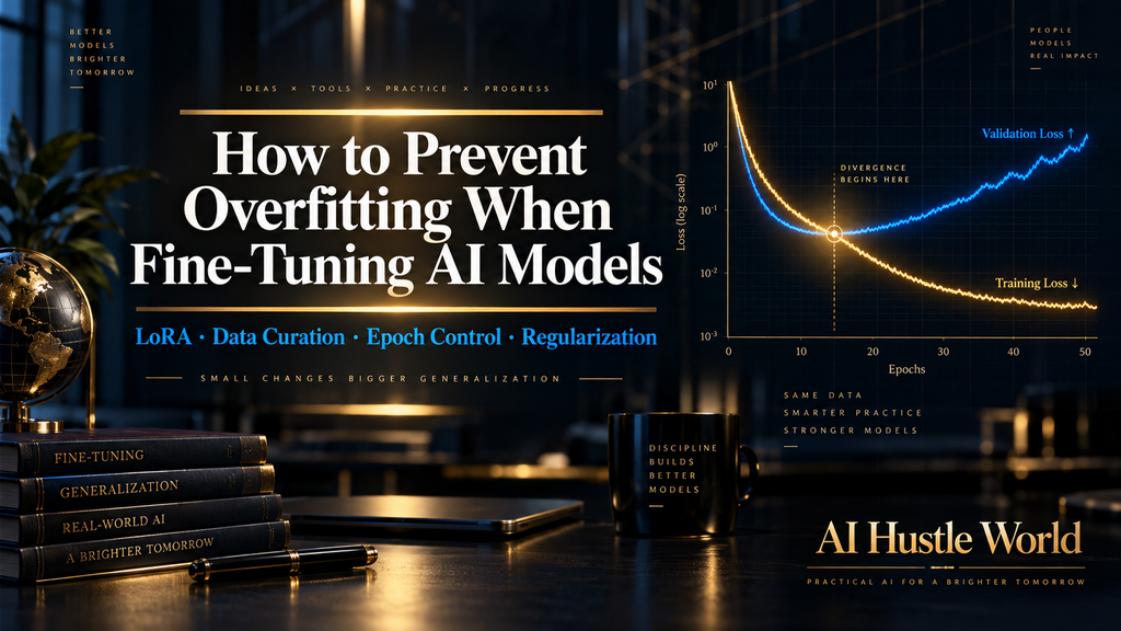
How to Prevent Overfitting When Fine-Tuning AI Models

How to Prevent Overfitting When Fine-Tuning AI Models

If you have ever fine-tuned a language model and watched it nail your test examples while falling apart on anything else, you have met overfitting. The model learned your data too well — and forgot how to generalize.

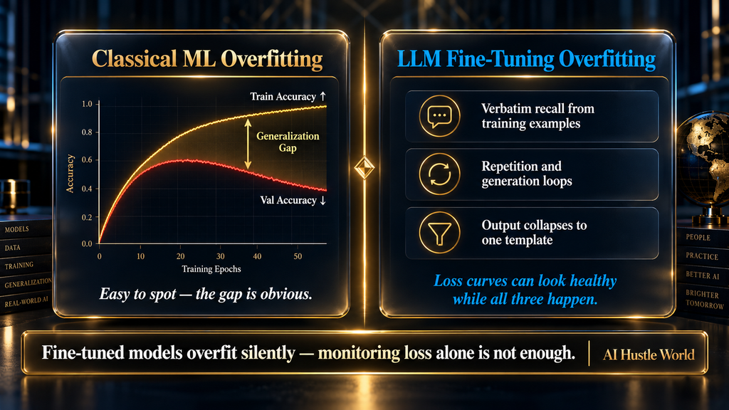
In classical machine learning, overfitting is straightforward to spot: training accuracy climbs while validation accuracy sags, and you stop training. With language models, the same divergence can still happen, but it often hides. The model passes your eval set, produces fluent text, and looks fine — until it starts echoing training answers verbatim, looping into repetition, or collapsing every response into a single template, regardless of what you asked. Loss curves can look reasonable right up until the model is deeply overfit.

This article covers what overfitting actually looks like in fine-tuned LLMs, why it happens, how to detect it before it costs you a training run, and the specific techniques — on the data side, the training side, and the architectural side — that reliably prevent it. If you are new to fine-tuning, start with Fine-Tuning AI Models Explained first. If your dataset is the issue, How to Prepare a High-Quality Dataset for Fine-Tuning a Language Model covers the preparation side in depth.

Quick Answer

Keep training to 1–3 epochs. Use LoRA instead of full fine-tuning. Curate a small, diverse, deduplicated dataset before you train. Monitor both training and validation loss together, and save checkpoints at every epoch so you can roll back. These four decisions prevent most overfitting failures in practice. Everything below explains why they work and when you need to go further.

What Overfitting Actually Means for a Fine-Tuned LLM

The classical definition of overfitting — the model memorizes training noise and fails on held-out data — still applies, but the way it shows up in a language model is different from what you see in a classifier or a regression model.

A fine-tuned LLM does not usually fail in an obvious way. It rarely drops 10 percentage points on a benchmark overnight. Instead, it starts returning verbatim training answers when users ask questions that share a prefix with something in the training set. It develops repetition loops — “the answer is the answer is the answer is…” — on familiar patterns. Its outputs narrow: instead of a range of phrasings, you get the same template every time. These are distributional collapse symptoms, and they are easy to miss if you are only watching loss.

The memorization research makes this concrete. Lee et al. found that in large language models, over one percent of unprompted output tokens are copied verbatim from training data. After deduplication of the training set, that figure dropped to roughly 0.1% — a tenfold reduction. In fine-tuning, where datasets are orders of magnitude smaller and you repeat the same examples across multiple epochs, memorization pressure is far stronger than in pretraining.

There is also an important distinction between memorization and overfitting. Tirumala et al. (arXiv:2205.10770) showed that LLMs begin memorizing individual training examples well before aggregate validation loss starts rising — which means you can have a model that is actively memorizing while your loss curve still looks healthy. The loss curve is a lagging indicator, not a real-time alert.

Why instruction fine-tuning is especially vulnerable. The LIMA paper (Zhou et al., NeurIPS 2023) advanced what they called the Superficial Alignment Hypothesis: essentially all of a model’s knowledge comes from pretraining, and instruction fine-tuning mostly teaches the model how to respond — style, format, register — rather than new factual knowledge.

If that is correct, the risk calculus changes. In full pretraining, you train on enormous, diverse data seen only once, so classical overfitting is nearly impossible. In instruction fine-tuning, you train on a small, narrow dataset repeated across multiple epochs.

If you push too hard — too many epochs, too high a learning rate, too narrow a distribution — you do not just fail to generalize. You actively overwrite pretrained knowledge. Full pretraining builds capability. Aggressive instruction fine-tuning erases it.

The Root Causes: Why Fine-Tuned Models Overfit

Understanding the cause matters because each prevention technique targets a specific root cause. They are not interchangeable.

Too many epochs is the most common cause. Most instruction-tuned models overfit within three to five epochs. The 1–3 epoch guidance is not arbitrary conservatism — it comes from repeated empirical observation that validation metrics plateau and then degrade past epoch 3 on typical instruction datasets. An F1 ablation study on multi-class classification found scores rising from one to three to five epochs, then falling at ten.

The caveat is that epoch tolerance is task-dependent. Teaching a model a genuinely new symbolic skill absent from pretraining may benefit from 20 to 30 epochs. But for the vast majority of instruction fine-tuning tasks — formatting, tone, domain vocabulary — three epochs is the ceiling.

Dataset quality and duplication amplify memorization. AlpaGasus (Chen et al., ICLR 2024) filtered Alpaca’s 52,000-example dataset down to 9,000 high-quality examples using ChatGPT-based auto-grading. The 9k-example model outperformed the full 52k model on downstream benchmarks — and trained seven times faster, cutting 7B training time from 80 minutes to 14 minutes.

Low-quality examples do not just waste compute; they teach the model noise patterns. Duplicates amplify those patterns across every epoch. Lee et al. found one 61-word sequence appearing 61,036 times in a training corpus. In a small fine-tuning dataset, a handful of near-duplicates repeated across three epochs behave exactly like that.

Narrow topic distribution limits generalization. QDIT (Bukharin & Zhao, EMNLP Findings 2024) showed that dataset diversity has a measurable, independent effect on model robustness: maximizing diversity in instruction selection improved worst-case performance by 18% while maintaining or improving average performance compared to quality-only selection baselines. A model fine-tuned on narrow data learns narrow behavior, and that behavior can look like overfitting when deployed on slightly different inputs.

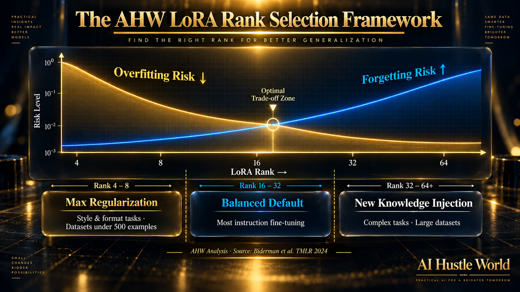
Full fine-tuning has far more capacity to overfit than LoRA. Biderman et al. (TMLR 2024) found that full fine-tuning learns weight perturbations with rank 10 to 100 times higher than typical LoRA configurations. That higher-rank update space gives full fine-tuning more room to fit the training distribution precisely — and more room to diverge from the base model’s pretrained distribution. LoRA’s rank constraint is not just an efficiency feature; it is a regularizer. If you need a full grounding on how LoRA works before continuing, LoRA Explained covers the mechanics in depth.

Learning rate too high for the amount of data. In pretraining, a high learning rate is tempered by enormous data diversity — every update encounters different examples, so no single pattern can dominate the gradient signal. In fine-tuning, that safeguard is absent. A high learning rate applied to a small, narrow dataset takes large, confident steps toward the training distribution’s local minimum before the model has had time to generalize. The gradient signal is homogeneous — it is repeating the same few hundred or few thousand examples — so large steps mean large movements toward memorization.

The practical consequence is asymmetric: a learning rate that would be fine for a 100,000-example dataset can cause visible memorization on a 500-example run. Typical ranges for instruction fine-tuning are 1e-5 to 5e-5 for full fine-tuning and 1e-4 to 2e-4 for LoRA. If you see repetition or template collapse within the first 100 to 200 steps, the learning rate is the first thing to reduce — cut it by 5× before changing anything else.

How to Detect Overfitting During Training

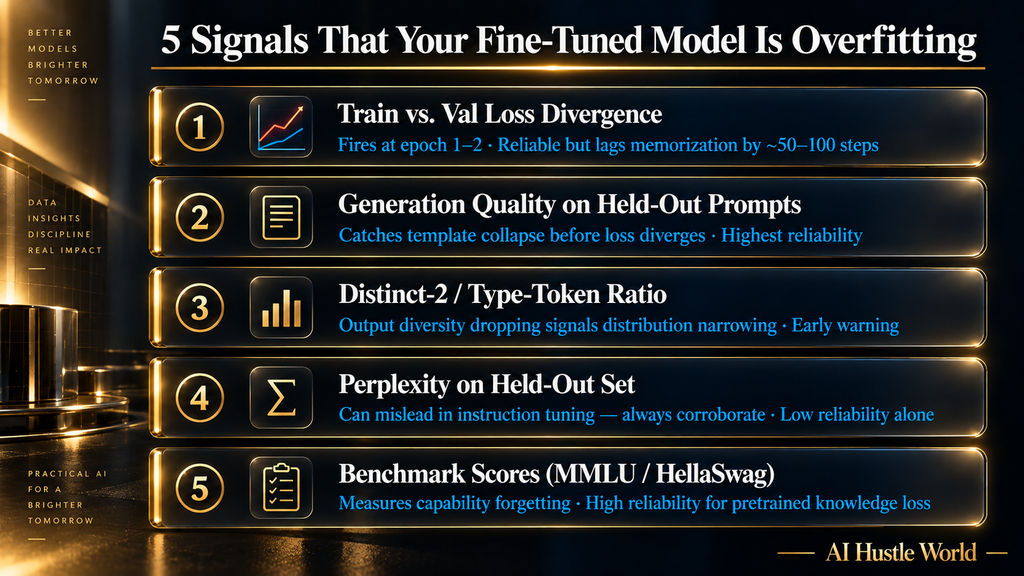
The earlier you detect overfitting, the cheaper the fix. Here are the signals to watch, in roughly the order of their reliability.

Training loss vs. validation loss divergence is the primary diagnostic. During healthy training, both losses decrease together, with validation loss slightly above training loss — a gap of around 0.1 to 0.2 is normal. The overfitting signal is when validation loss plateaus or begins rising while training loss keeps dropping. On a typical 3-epoch run, the inflection often appears between epoch 1 and epoch 2. If you see validation loss rising after epoch 1, stop at epoch 1.

Generation quality on held-out prompts. Loss divergence is a lagging indicator; generation quality can degrade earlier. Build a callback that samples the model on 20 to 50 held-out prompts every 200 to 500 steps and logs the outputs. In Hugging Face Trainer, this is a TrainerCallback with an on_evaluate method that runs model.generate() with do_sample=True, temperature=0.7, max_new_tokens=256 and writes outputs to a file or a W&B/MLflow run.

Look for three signals: outputs becoming repetitive across different prompts, outputs collapsing into a single template structure regardless of input, and outputs echoing verbatim phrasing from training examples. These typically appear 50 to 100 steps before the loss curves diverge visibly.

Output diversity metrics. Distinct-n measures the ratio of distinct n-grams to total n-grams in a set of generated responses — a model that has collapsed to a narrow output distribution produces fewer unique bigrams and trigrams. A dropping distinct-2 score across checkpoints is a reliable early warning that the model’s generation distribution is narrowing.

You can compute it with a few lines of Python: tokenize a batch of generated responses, count unique bigrams and total bigrams, divide. Type-token ratio (TTR) — unique tokens divided by total tokens — serves the same purpose and is simpler to compute. Both are most useful for comparison across checkpoints, not as absolute thresholds; implement them in the same callback that logs generation samples.

A critical caveat on perplexity. Perplexity on a held-out set is a standard tool, but LIMA demonstrated that in alignment fine-tuning, perplexity can negatively correlate with generation quality. As training continued past the early checkpoints in their 15-epoch run, held-out perplexity rose — a classic overfitting sign — but human evaluators actually preferred the later-checkpoint generations. LIMA’s solution was to select their final checkpoint manually from a 50-example dev set, because perplexity alone was misleading. Do not early-stop on perplexity alone for instruction-style fine-tuning.

Benchmark-level signals. For any run where capability retention matters, track performance on source-domain benchmarks — MMLU, HellaSwag, WinoGrande, ARC-Challenge — at each checkpoint using the EleutherAI LM Evaluation Harness. A drop of more than 2 to 3 points on MMLU or HellaSwag from the base model is a forgetting signal, not just an overfitting signal, and means you are eroding pretrained knowledge. The Harness is the backend for Hugging Face’s Open LLM Leaderboard, runs on 60+ standardized tasks, and lets you compare your local checkpoint directly against published results.

Early stopping configuration. In Hugging Face Trainer, EarlyStoppingCallback with patience 3 and min_delta ~0.001 on eval_loss is a reasonable starting point. Use load_best_model_at_end=True with metric_for_best_model="eval_loss". One practical note: with 4-bit quantized training (QLoRA), quantization noise makes the loss noisier, so increasing patience to 5 helps avoid false stops. Also check your Transformers version — in 4.30.0+, early_stopping_threshold was changed from absolute delta to a relative percentage.

Here is how the five detection signals compare in practice:

Signal	What It Catches	When It Fires	Reliability	How to Compute
Train vs. val loss divergence	Memorization pressure	Epoch 1–2 inflection	High — but lags memorization onset	Built into Trainer logs
Generation quality review	Template collapse, verbatim echo	50–100 steps before loss diverges	Highest — catches what loss misses	Manual or callback sampling
Distinct-2 / TTR	Output distribution narrowing	Early, even with stable loss	Good for trend tracking	Python: unique bigrams ÷ total bigrams
Perplexity on held-out set	General overfitting	Epoch boundary	Low for instruction tuning (can mislead)	Built into Trainer eval
Benchmark scores (MMLU etc.)	Capability forgetting	Across epochs	High for forgetting, not for collapse	EleutherAI LM Eval Harness

Prevention: The Data Side

Fixing your data prevents more overfitting than any training hyperparameter. This is the counterintuitive lesson from the LIMA and AlpaGasus papers: the training regime matters far less than the quality and diversity of what you train on.

Curate, do not just collect. LIMA achieved strong alignment on 1,000 carefully selected examples — 750 high-quality answers from Stack Exchange and wikiHow selected for quality and diversity, plus 250 manually written examples, roughly 750,000 tokens total. AlpaGasus showed that 9,000 filtered examples outperformed 52,000 unfiltered ones.

The pattern is consistent: a smaller, well-curated dataset generalizes better than a larger, noisier one. For most domain-specific enterprise fine-tuning tasks, performance plateaus around 500 to 600 high-quality examples (arXiv:2503.01870). If a task saturates at 600 examples, collecting 6,000 more of the same type is counterproductive — you get more memorization, not more generalization.

Deduplicate before training. Exact and near-duplicate removal is not optional. Lee et al. (ACL 2022) showed that deduplication reduced verbatim memorized token emissions by roughly tenfold, and that over 4% of standard validation splits contained examples that also appeared in the training set — making eval metrics optimistic. Use exact hash deduplication as the first pass, then MinHash with LSH for near-duplicate detection. If you built your dataset following the guidance in How to Prepare a High-Quality Dataset for Fine-Tuning a Language Model, deduplication should already be done before training starts.

Maximize diversity, not just quality. QDIT’s +18% worst-case robustness improvement came from diversity selection alone, independent of quality filtering. Practically, this means maximizing the breadth of tasks, phrasings, topics, and response lengths in your training set. A fine-tuned model that has only seen one style of user question will overfit to that style and fail when the phrasing shifts.

Multi-task mixing for domain fine-tuning. If you are fine-tuning on a narrow domain, mix in a proportion of general instruction-following data. This acts as a regularizer at the data level: the model cannot collapse to narrow domain behavior if it is also being trained to answer general questions. A practical starting proportion is 10 to 20% general instruction data — enough to anchor broad behavior without diluting domain-specific performance. Above 30%, you start reducing the domain signal meaningfully; below 5%, the mixing effect is minimal.

Luo et al. found that models with prior general instruction tuning forgot less during subsequent domain fine-tuning than models that went from raw base to domain fine-tune directly. This suggests that even a prior general-instruction stage — before domain fine-tuning begins — provides forgetting resistance independently of in-batch mixing.

Prevention: The Training Side

Once the data is in good shape, the training configuration is the next lever.

Keep epochs to 1–3. For style and format instruction fine-tuning — the most common use case — the model learns the target behavior within the first one or two passes through the data. Additional epochs increase memorization without improving generalization. The specific advice for your run: if your training loss has plateaued and validation loss is flat or rising after epoch 2, stop. Do not run epoch 3 out of habit.

Learning rate and scheduling. A warmup period followed by cosine decay is the standard for longer runs (3+ epochs). For short runs (1–2 epochs), linear decay is often sufficient. LIMA’s specific configuration is instructive: no warmup, initial learning rate of 1e-5 decaying linearly to 1e-6, batch size 32, weight decay 0.1, AdamW (β1=0.9, β2=0.95). For LoRA fine-tuning, 2e-4 is a common starting point. If you see repetition or looping within the first 100 steps, the learning rate is too high — reduce by 2 to 5×.

Weight decay. L2 regularization through weight decay (0.01 to 0.1) penalizes large weight magnitudes and prevents the model from committing too strongly to any particular training signal. It is the least expensive regularizer to add and should be enabled by default. LIMA used 0.1; most LoRA runs use 0.01 to 0.05.

Gradient clipping. Clip gradients to a maximum norm (1.0 is common) to prevent large, destabilizing updates — particularly useful in early training steps and when working with quantized models. It does not prevent overfitting directly, but it prevents the training run from drifting into instability that can masquerade as overfitting.

Dropout — and when to enable it. Dropout is disabled by default in most transformer implementations, and for good reason: it can hurt convergence in large models when not tuned carefully. LIMA used residual dropout ramping from 0.0 at the bottom layer to 0.3 at the top layer (0.2 for smaller models). If you see strong memorization symptoms and weight decay alone is not enough, adding 0.1 dropout to attention layers is a reasonable next step.

Save checkpoints at every epoch. This is not optional. LIMA trained for 15 epochs and selected its final checkpoint from between epochs 5 and 10 based on a 50-example dev set — not from the final epoch. You cannot roll back if you did not save. Set save_strategy="epoch" and keep the top 3 checkpoints by eval loss.

Prevention: LoRA and PEFT as Structural Regularizers

Using a parameter-efficient fine-tuning method like LoRA is not just an efficiency choice. It is, in many situations, the most powerful overfitting prevention tool available.

Why LoRA resists overfitting. LoRA (Hu et al., ICLR 2022) freezes the pretrained weights and injects trainable low-rank decomposition matrices into the attention layers. Trainable parameters drop by up to 10,000× compared to full fine-tuning of GPT-3-scale models.

Biderman et al. (TMLR 2024) ran the critical comparison: full fine-tuning learns weight perturbations with rank 10 to 100 times higher than typical LoRA configurations. That high-rank update space is what allows full fine-tuning to fit the training distribution so tightly.

LoRA’s rank constraint limits the model’s capacity to overfit. Biderman et al. found it provides stronger regularization than weight decay or dropout — not just comparable. It also produces more diverse generations as a direct result.

Choosing rank. The original LoRA paper showed that a rank as low as 1 or 2 can be sufficient even when the full weight dimension is 12,288. Common practical ranges are rank 8 to 64. Lower rank = stronger regularization and less forgetting, because the update is confined to a smaller subspace. For most instruction fine-tuning tasks, start at rank 16. If you see memorization symptoms, drop to rank 8. If you are injecting genuinely new knowledge (not just adjusting style), rank 32 to 64 may be needed to provide enough capacity.

LoRA dropout. Lin et al. introduced LoRA Dropout as a sparsity regularizer with a proven generalization-error bound. It functions like standard dropout but applied to the LoRA adapters, improving both accuracy and calibration. A starting value of 0.05 to 0.1 is practical for most runs. Note that some base models (like Mistral) have internal dropout in their attention layers, so check before stacking additional dropout.

QLoRA for memory-constrained setups. Dettmers et al. (NeurIPS 2023) combined 4-bit NormalFloat (NF4) quantization of the frozen base model with standard LoRA adapters in 16-bit precision. QLoRA enables fine-tuning a 65B-parameter model on a single 48GB GPU while preserving 16-bit fine-tuning performance — and because it is still LoRA under the hood, the regularization properties carry over. The Guanaco models trained with QLoRA reached 99.3% of ChatGPT performance on the Vicuna benchmark in 24 hours on a single GPU.

Other PEFT options. For extreme parameter efficiency, IA³ (Liu et al.) rescales inner activations using learned vectors, using roughly 0.01 to 0.02% of model parameters. It was the only PEFT method in its study to outperform full fine-tuning in the few-shot setting. Prompt tuning (Lester et al.) prepends learned continuous embeddings, using less than 0.01% of parameters — but its quality only matches full fine-tuning at 10B+ parameter scale, making it impractical for most smaller fine-tuning tasks.

For most practitioners, LoRA at rank 8 to 16 is the right default. It handles the majority of instruction fine-tuning use cases, trains faster, requires less GPU memory, and regularizes more aggressively than full fine-tuning with dropout and weight decay.

Prevention: Additional Regularization Techniques

Beyond epochs, data curation, and LoRA, several targeted regularization techniques address specific failure modes.

Label smoothing (Müller, Kornblith & Hinton, arXiv:1906.02629, NeurIPS 2019) softens the one-hot training targets — instead of training the model to assign 100% probability to the correct token, it assigns (1 – ε) to the correct token and distributes ε uniformly across the vocabulary (ε = 0.1 is standard). This prevents the model from becoming overconfident in its predictions, which is a form of memorization. A critical caveat from the same paper: label smoothing hurts knowledge distillation — if your fine-tuning pipeline uses a teacher model’s logits, do not apply label smoothing to those targets.

KL-divergence penalty. Adding a KL divergence term between the fine-tuned model’s output distribution and the frozen base model’s output distribution penalizes the model for drifting too far from what it already knew. This is built into DPO’s β parameter, but it can also be implemented in standard supervised fine-tuning. The implementation involves running a frozen copy of the base model as a reference policy: for each training batch, compute log probabilities of the target tokens under both the reference model and the current model, then add λ × KL(π_θ || π_ref) to your cross-entropy loss.

A λ value of 0.1 to 0.5 is a typical starting range — larger λ anchors more strongly to the base, smaller λ allows more adaptation. The main cost is memory: a second model copy doubles GPU memory consumption. If that is prohibitive, DPO with a higher β achieves the same anchoring effect more efficiently, since it does not require a separate generation step.

DPO as an alignment alternative. For behavior alignment tasks — where you want the model to prefer certain response styles over others — Direct Preference Optimization (Rafailov et al., NeurIPS 2023) is worth considering over pure supervised fine-tuning. DPO’s β parameter (default 0.1 in Hugging Face TRL) controls how far the policy can drift from the reference model via a KL penalty. Higher β anchors the model more strongly to the base; lower β allows more adaptation. DPO also reduces catastrophic forgetting compared to naive SFT in most benchmark comparisons.

Here is how the main prevention techniques compare across the dimensions that matter most for a practical fine-tuning decision:

Technique	Overfitting Prevention	Forgetting Prevention	Implementation Complexity	Best For
LoRA (rank 8–16)	Very high	High	Low	Most instruction fine-tuning tasks
Full fine-tuning + weight decay	Medium	Low	Low	Large datasets (5k+ examples)
Epoch reduction (1–2 epochs)	High	Medium	None	Any run showing val loss rise
Data deduplication	High	Medium	Low	All datasets — do this first
Label smoothing (ε = 0.1)	Medium	Low	Low	High-confidence memorization risk
LoRA dropout (0.05–0.1)	Medium–High	Low	Low	LoRA runs with small datasets
KL divergence penalty	Medium	High	High (needs reference model)	Alignment tasks, style fine-tuning
DPO (β = 0.1–0.5)	Medium	High	Medium	Preference alignment over naive SFT
Multi-task mixing (10–20%)	Medium	High	Low	Narrow domain fine-tuning
EWC	Low–Medium	Very high	Very high	Continual/sequential fine-tuning

Catastrophic Forgetting: The Related Problem

Overfitting and catastrophic forgetting are related but distinct. Overfitting is fitting the training set too tightly. Catastrophic forgetting is losing previously learned capabilities as new ones are acquired. They frequently co-occur during aggressive fine-tuning, and the prevention strategies overlap significantly.

Luo et al. measured forgetting empirically across 1B to 7B models during continual instruction fine-tuning. They found it is general across model sizes and intensifies with scale — larger models start with higher base capability and lose more of it when aggressively fine-tuned. Decoder-only models like the LLAMA family forgot more than encoder-decoder models.

Critically, models with prior general instruction tuning forgot less during subsequent domain fine-tuning. That argues for a multi-stage approach: general instruction tuning first, then domain adaptation.

More recent work traced catastrophic forgetting in LLMs to “intruder dimensions” — high-magnitude singular vectors in the update matrix that overwrite pretrained directions. Low-rank updates like LoRA minimize these intruder dimensions, which is another mechanistic explanation for why LoRA forgets less. Biderman et al. confirmed this empirically: in their comparison, the extent of forgetting was inversely related to LoRA rank — lower rank preserved more base capability.

That same research traced catastrophic forgetting in LLMs to what the authors called “intruder dimensions” — high-magnitude singular vectors that appear in the weight update matrix and overwrite pretrained representational directions. When you fine-tune aggressively, the update matrix ΔW develops a few dominant singular vectors with very large magnitudes.

These intruder dimensions effectively hijack the directions in weight space that the base model had learned to associate with general capabilities, replacing them with fine-tuned task representations. Low-rank updates like LoRA constrain the rank of ΔW, which limits how many such intruder dimensions can form. This is a second mechanistic reason — beyond parameter count — for why LoRA forgets less.

Elastic Weight Consolidation (Kirkpatrick et al., PNAS 2017) provides a more explicit forgetting-prevention mechanism. EWC adds a quadratic penalty to the loss function, weighted by the Fisher information matrix of the original task. The Fisher information captures which weights were most important for prior performance — weights with high Fisher information get penalized heavily if they change, while less important weights can adapt freely. The effect is that the model can learn new task behavior while being constrained to keep the weights that matter most for what it already knew.

In practice, EWC is complex to implement correctly. Computing the Fisher information matrix requires a forward pass over a representative reference dataset, and the full Fisher matrix is too large to store for modern LLMs — diagonal approximations are used instead, which reduces accuracy.

EWC is most useful in continual learning settings where you fine-tune on a sequence of tasks over time and cannot afford to replay old training data. For a single-domain fine-tuning job — the most common case — LoRA at low rank combined with 10 to 20% general instruction data mixing provides comparable forgetting resistance with far less implementation overhead.

A Practical Decision Framework

The right prevention strategy depends on your dataset size. Use this table as your starting configuration, then adjust based on what you observe during training.

Dataset Size	Method	Rank	Epochs	Weight Decay	Extra Regularization	Monitor
Under 300 examples	Consider RAG first	—	—	—	—	—
300–500 examples	LoRA	4–8	1–2	0.1	LoRA dropout 0.1, manual gen review	Generation quality every checkpoint
500–5,000 examples	LoRA	16–32	2–3	0.05	Early stopping (patience 3)	Train/val loss + generation samples
5,000–50,000 examples	LoRA or full FT	32–64	2–3	0.01–0.05	Warmup + cosine decay	MMLU/HellaSwag at each epoch
50,000+ examples	Full fine-tuning	—	1–3	0.01	Gradient clipping (norm 1.0)	Benchmark suite + val loss

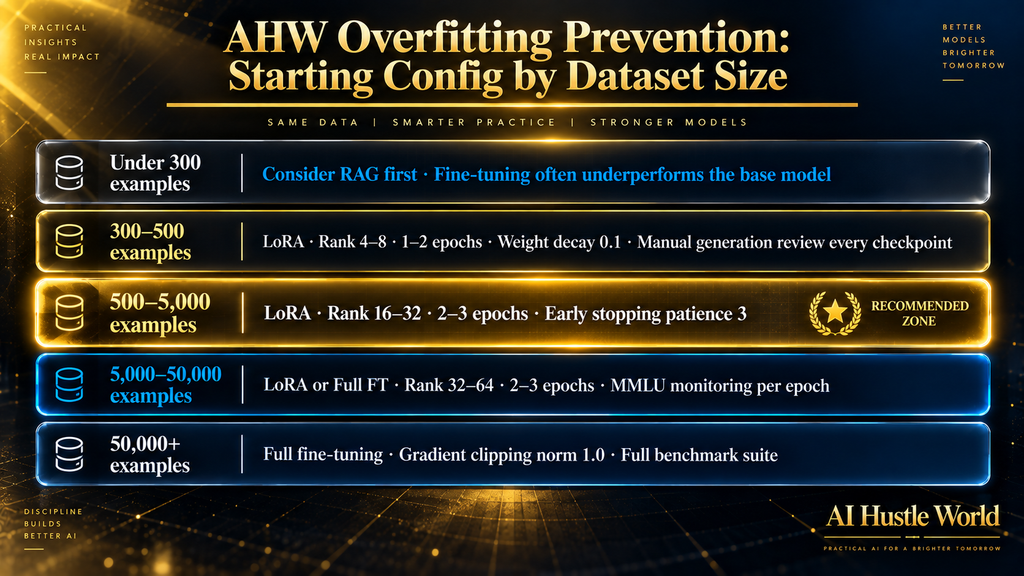
Below 300 examples, fine-tuning frequently fails to improve over the base model for tasks the base already handles — retrieval-augmented generation is often a better investment. Above 5,000 examples, full fine-tuning becomes viable, but LoRA is still the safer default for capability retention unless you have a specific reason to update all weights.

Signs your model has overfit:

• Outputs repeat phrasing or sentence structures that appear in training examples
• The model passes your evaluation set but fails on production-mirror prompts with different phrasing
• MMLU or HellaSwag score dropped more than 2 to 3 points from the base model baseline
• Output distinct-2 score is declining across checkpoints while validation loss looks stable
• The model gives narrow refusals or a single templated response on tasks it handled correctly before fine-tuning
• Outputs loop or terminate prematurely in a pattern not present in the base model

Common Mistakes

Running the full epoch count by default. Three epochs is a default, not a target. Most practitioners set num_train_epochs=3 at the start of a run and let it finish regardless of what the validation curve shows. The problem is that the right epoch count depends on your data size, diversity, and task — and for most instruction fine-tuning on datasets under 2,000 examples, the model has already learned what it needs to learn by the end of epoch 1. Epoch 2 and 3 just reinforce the training distribution more deeply. If validation loss is rising after epoch 1, stopping at epoch 1 is the correct decision. The checkpoint you want is the best checkpoint, not the final one. This is why save_strategy="epoch" and load_best_model_at_end=True should be non-negotiable defaults.

Trusting only the loss curve. This is the most dangerous mistake because it looks like due diligence. You are monitoring training — the loss curves look reasonable — so you proceed to deploy. But validation loss can be flat or gently declining while the model is simultaneously memorizing training phrasing, narrowing its output distribution, and quietly dropping 3 points on MMLU.

Loss measures average cross-entropy across the eval set. It does not measure whether outputs are parroting training data, whether generations have collapsed to one template, or whether the model can still do things it could do before fine-tuning. Always corroborate loss with generation samples on held-out prompts and, for capability-sensitive tasks, source-domain benchmark scores.

Skipping deduplication because the dataset feels small. There is a widespread assumption that deduplication matters at the pretraining scale but is unnecessary for a 500 or 1,000-example fine-tuning set. This is backward. A 1,000-example dataset with 50 near-duplicate pairs, run for 3 epochs, trains on those 50 pairs effectively 6 times relative to the rest of the dataset.

The model does not average those examples out — it amplifies them. The duplicated patterns get disproportionately reinforced, and the model starts reproducing them preferentially. Lee et al. showed the effect even at pretraining scale: one 61-word sequence appeared 61,036 times and was memorized near-perfectly. The same dynamic operates at fine-tuning scale, just with a much smaller dataset where each duplicate has far more relative weight.

Adding more data to fix overfitting. When a model starts memorizing or collapsing, the instinct is to collect more examples and retrain. If the new data comes from the same narrow distribution — the same topics, the same phrasing patterns, the same response templates — this makes the memorization worse, not better. The model now has more examples of the same thing to memorize.

The fix is not volume; it is diversity. Adding 500 examples from a different task domain, different response lengths, and different phrasing styles does more to prevent overfitting than adding 5,000 more examples from the same source.

Using full fine-tuning when LoRA would work. Full fine-tuning updates every parameter in the model, giving it maximum capacity to fit the training distribution — and maximum capacity to overfit it. For the vast majority of instruction-style tasks — adjusting format, tone, domain vocabulary, response style — that capacity is unnecessary. LoRA at rank 16 matches or outperforms full fine-tuning on most instruction benchmarks while regularizing more aggressively, using a fraction of the GPU memory, and preserving more pretrained capability. Biderman et al.

Found that full fine-tuning’s forgetting was substantially higher than LoRA’s at every rank they tested. Full fine-tuning is warranted when you are injecting genuinely new knowledge absent from pretraining, or when you need to modify the model’s behavior at a depth that low-rank updates cannot reach. For everything else, it is the wrong default.

Setting the same learning rate for LoRA and full fine-tuning. LoRA adapters start from near-zero initialization and need higher learning rates to converge — typically 1e-4 to 2e-4. Full fine-tuning starts from already-trained weights and needs much lower rates to avoid destroying them — typically 1e-5 to 5e-5. Using a full fine-tuning learning rate on LoRA causes slow convergence; using a LoRA learning rate on full fine-tuning causes rapid memorization and forgetting. This is one of the most common hyperparameter mistakes in fine-tuning tutorials that copy configs without explanation.

The AHW Overfitting Prevention Hierarchy

One pattern runs consistently through the research on LLM fine-tuning overfitting: the interventions that work most are structural, not numerical. Practitioners often reach for hyperparameter tuning — lowering the learning rate, adding more dropout — when the real fix is upstream in the architecture or the data.

Based on the research surveyed here, the effective prevention hierarchy runs in this order: (1) dataset quality and deduplication, (2) architecture choice (LoRA vs. full fine-tuning), (3) epoch count, (4) training-side regularization (weight decay, early stopping), (5) advanced techniques (label smoothing, KL penalty, LoRA dropout). Most failed fine-tuning runs are stuck on step 4 or 5 while steps 1 and 2 were never addressed.

The practical implication: if your model is overfitting and you are reaching for dropout values, check whether your dataset has duplicates and whether you are using full fine-tuning when LoRA would do. Those two decisions have more leverage than any regularization parameter.

Final Thoughts

The central finding from the research is consistently counterintuitive: less training, on smaller but better data, with fewer trainable parameters, almost always outperforms the alternative. LIMA beat models trained on 52× more examples. AlpaGasus beat Alpaca using 9,000 examples filtered from 52,000. LoRA regularizes more strongly than weight decay and dropout while using a fraction of the parameters.

Most overfitting in fine-tuning is not a training problem — it is a data problem followed by a training configuration problem. Fix the data first: deduplicate, filter for quality, maximize diversity, right-size for the task. Then use LoRA at an appropriate rank, limit epochs to 1–3, save checkpoints, and monitor validation loss and generation quality together.

Where more is needed — small datasets, aggressive domain adaptation, multi-stage fine-tuning — the techniques in this article (LoRA dropout, label smoothing, KL penalty, general-instruction mixing, manual checkpoint selection) provide a clear escalation path. The goal throughout is the same: a model that learned your target behavior without forgetting everything else.

FAQ

What is overfitting in fine-tuning?

It is when a model learns the training data too precisely and fails to generalize. In LLMs, this shows up as verbatim recall, repetition loops, and collapsed output diversity rather than the classic train/test accuracy gap.

How many epochs should I train to avoid overfitting?

1 to 3 epochs for most instruction fine-tuning tasks. Stop at the checkpoint with the lowest validation loss, not necessarily the final epoch.

Does LoRA prevent overfitting?

Yes, inherently. LoRA’s rank constraint limits the parameter space, providing regularization that Biderman et al. found is stronger than weight decay or dropout in practice.

What is the difference between overfitting and catastrophic forgetting?

Overfitting is fitting the training set too tightly. Catastrophic forgetting is losing pretrained capabilities. They often occur together during aggressive fine-tuning, but require slightly different fixes — LoRA and data diversity address both.

How do I detect overfitting early?

Watch training vs. validation loss divergence, review generation outputs at each checkpoint, and track output diversity metrics (distinct-n). Validation loss rising while training loss drops is the clearest signal.

Is perplexity a reliable overfitting signal for LLMs?

Not always. LIMA showed perplexity can negatively correlate with generation quality in instruction fine-tuning. Always corroborate perplexity with generation review.

What weight decay value should I use?

0.01 to 0.1 is the practical range. LIMA used 0.1. Most LoRA runs use 0.01 to 0.05. Start at 0.01 and increase if you see memorization symptoms.

What LoRA rank should I use?

Rank 8 to 16 for most instruction fine-tuning tasks. Lower rank = more regularization and less forgetting. Increase to 32 to 64 only if you are injecting genuinely new knowledge rather than adjusting style.

Can I fine-tune on fewer than 500 examples without overfitting?

Yes, with LoRA at low rank, 1 to 2 epochs, high weight decay, and diverse examples. Below roughly 300 examples, check whether RAG is a better fit before investing in fine-tuning.

What is early stopping and should I use it?

Early stopping halts training when validation loss stops improving (with a patience parameter). It is strongly recommended for any run of 2+ epochs. Use EarlyStoppingCallback in Hugging Face Trainer with patience 3 and load_best_model_at_end=True.

Related Guides

• How AI Learns From Data: A Complete Beginner’s Guide
• Few-Shot vs Zero-Shot Prompting: When Should You Use Each?
• How to Detect and Reduce Bias in AI-Assisted Decision Making