Fine-Tuning AI Models Explained: Full Fine-Tuning, LoRA and When to Use Each

Fine-Tuning AI Models Explained: Full Fine-Tuning, LoRA and When Each Approach Actually Makes Sense

Most people who ask about fine-tuning AI models are actually asking three different questions at once without realizing it. The first question is whether they should fine-tune at all — or whether a well-engineered prompt or a retrieval system would solve the problem faster and cheaper. The second question is which fine-tuning method fits their specific hardware and goal. The third question is what their training data actually needs to look like.

Most explanations treat these as a single flat decision: “fine-tuning vs LoRA.” They’re not. They’re sequential. And the order matters, because committing to the wrong step — especially skipping the first question — is how practitioners end up spending hundreds of dollars on a training run that a better system prompt would have made unnecessary.

This article walks through each question in sequence, with concrete hardware numbers, real dataset thresholds, and the research findings that most competing guides never mention. By the end, you’ll have a structured decision framework you can apply to any fine-tuning scenario — not just the theory of how fine-tuning works.

One boundary up front: this article doesn’t cover fine-tuning code, dataset preparation workflows, or LoRA hyperparameter tuning in depth — for those, see our LoRA guide, dataset preparation guide and guide to preventing overfitting. This is the decision layer: what to understand and verify before you commit to a method.

The Quick Answer: Which Approach Should You Use?

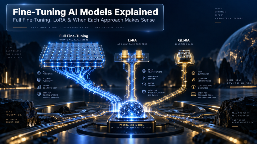
Fine-tuning adapts a pre-trained AI model to your specific task by continuing its training on your own data — updating either all its weights (full fine-tuning) or only a small set of low-rank adapter matrices (LoRA). Full fine-tuning produces deeper behavioral changes but requires enormous GPU resources. LoRA achieves comparable results on most single-task scenarios at a fraction of the cost.

QLoRA — which quantizes the base model to 4-bit and adds LoRA adapters — brings the hardware floor down to a single consumer GPU. The right choice depends on three factors: what you’re trying to change, what hardware you actually have, and how much quality training data you can prepare.

What Is Fine-Tuning? (And What It Isn’t)

Fine-tuning is the process of continuing to train a pre-trained language model on a new, task-specific dataset so that it updates its internal weights to better serve a particular purpose. That definition contains an important phrase: “continuing to train.” A base model like Llama 3 or Mistral has already been trained on hundreds of billions of tokens from the internet, books, and code. That training encoded an enormous amount of general knowledge into the model’s parameters. Fine-tuning doesn’t erase that knowledge — it nudges the model’s behavior in a new direction while building on what’s already there.

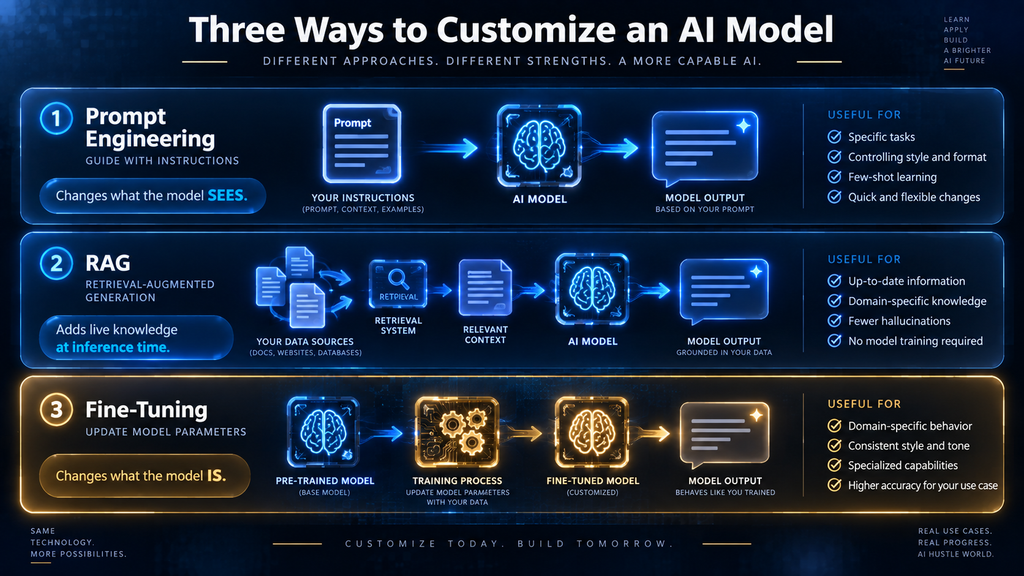
What fine-tuning is not: it is not the same as prompt engineering, which gives the model instructions but changes nothing in its weights. It is not the same as retrieval-augmented generation (RAG), which keeps the model frozen and gives it external documents to reference at inference time. Both of those approaches change what the model sees — fine-tuning changes what the model is. That distinction determines what problems each approach can actually solve.

Prompt engineering and RAG handle dynamic knowledge well — facts that change, documents that update, user-specific data that varies by session. Fine-tuning handles behavioral change — consistent output style, specialized vocabulary, structured formats, or domain-adapted reasoning that should be present on every single response without needing an elaborate prompt to trigger it every time. If you can get the behavior you want through a good system prompt and a few examples, fine-tuning is almost certainly the wrong tool for the job.

For a foundation on how pre-trained models learn in the first place, How AI Learns from Data: A Complete Beginner’s Guide covers the training mechanics that fine-tuning builds on. If you’re still deciding whether fine-tuning or RAG is the right paradigm for your use case, RAG vs Fine-Tuning: Which Approach Should You Use? covers that decision directly. This article assumes you’ve already concluded that fine-tuning is the right path — and focuses on which fine-tuning method and what you actually need to make it work.

How Full Fine-Tuning Works

Full fine-tuning updates every single parameter in the model during training. When you run a fine-tuning pass, gradients flow backward through all the transformer layers, and every weight matrix gets adjusted based on the loss computed from your training examples. Nothing is frozen — the entire model is in play.

This is powerful because it lets the model change at a fundamental level. When you need the model to not just know a new domain but reason differently within it — to produce outputs that are structurally different from its base behavior — full fine-tuning gives you that depth. Large-scale behavioral change, multi-domain adaptation, and cases where lower-cost methods have already plateaued are the natural territory for full fine-tuning.

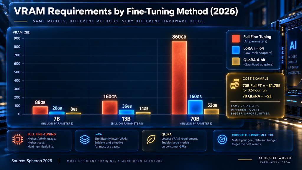
The cost is what makes full fine-tuning impractical for most practitioners. Training a 7B parameter model with full fine-tuning requires approximately 88 GB of VRAM just to hold model weights, optimizer states, and gradients simultaneously — that’s at least two H100 80 GB cards. A 70B model requires roughly 860 GB, which means eleven H100 SXM5 cards running in parallel for the full training duration.

At approximately $3.00–$3.50 per GPU hour per H100, a 32-hour fine-tuning run for a 70B model lands around $1,785 in compute costs, before data preparation time and the iterations typically needed to get the run right. These figures come from Spheron’s 2026 GPU compute analysis and represent real-world costs, not theoretical minimums.

Full fine-tuning is also the most susceptible to catastrophic forgetting — a failure mode covered in detail later — precisely because every parameter is in play simultaneously. The more weights you update aggressively, the greater the risk that previously encoded knowledge gets overwritten by the new domain data.

How LoRA Works

LoRA (Low-Rank Adaptation) is a parameter-efficient fine-tuning technique introduced by Hu, Shen, Wallis, Allen-Zhu, Li, Wang, Wang, and Chen (2021) that reduces the number of trainable parameters by decomposing weight updates into two small matrices instead of modifying the full weight matrices directly. The base model weights stay completely frozen throughout training. Only the small adapter matrices are updated. At inference time, the adapter outputs are added directly to the frozen base model outputs, so there’s no runtime penalty if you merge the adapters after training.

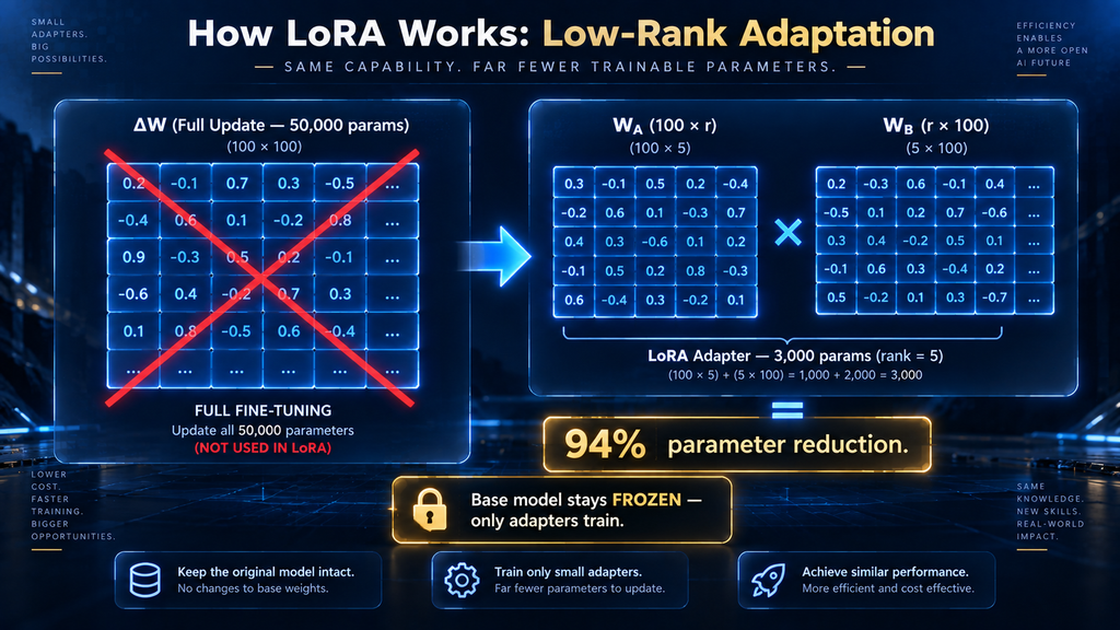
Here is the core mechanic: when you fine-tune a model, you’re effectively computing a change matrix ΔW — the difference between the original weights and what they should become. For a standard weight matrix, ΔW has the same dimensions as the original matrix, which can mean tens of millions of parameters per layer. LoRA observes that the meaningful portion of ΔW during fine-tuning tends to be low-rank — it can be well-approximated by two much smaller matrices multiplied together. Specifically, LoRA writes ΔW ≈ W_A × W_B, where W_A has dimensions (d × r) and W_B has dimensions (r × d), and r (the “rank”) is a small integer — typically 4, 8, or 16.

The parameter reduction is substantial. For a weight matrix of 100 × 500 (50,000 parameters), a full ΔW also requires 50,000 parameters. With LoRA at rank 5, you have a 100×5 matrix (500 parameters) and a 5×500 matrix (2,500 parameters) — just 3,000 parameters total, a 94% reduction. In 2023, Sebastian Raschka benchmarked LoRA at rank 8 applied to a LLaMA 7B model and found the resulting adapter was approximately 8 MB — compared to 23 GB for the full model weights.

That compact adapter size is also what makes LoRA practical for multi-tenant deployment: you can host one base model and swap different adapters for different customers or use cases without running separate full model instances.

The Rank Hyperparameter

The rank r controls how many parameters the LoRA adapters use and how expressive they can be. Higher rank means more parameters, more capacity to capture complex behavioral changes, and more VRAM required. Lower rank is more efficient but may not be sufficient for tasks that require deeper behavioral shifts.

For most practical use cases, r=4 to r=8 is the right starting point. Style and format consistency work well at r=4. Structured output and domain vocabulary tasks typically benefit from r=8 to r=16. Deep domain adaptation in specialized fields — medical, legal, highly technical — may need r=32 or higher. The right rank is almost always determined empirically through validation loss curves rather than chosen theoretically upfront, because the optimal rank depends on both your task complexity and your data distribution.

QLoRA: The Practical Middle Ground

QLoRA (Quantized LoRA), introduced by Dettmers, Pagnoni, Holtzman, and Zettlemoyer (2023), takes LoRA’s adapter-only training and adds one more layer of efficiency: it quantizes the frozen base model weights to 4-bit precision before training begins. The adapter matrices themselves stay in full precision (bfloat16 or float32), but the base model uses only 4 bits per parameter instead of 16.

The VRAM impact is dramatic. A 7B model that requires 88 GB for full fine-tuning and roughly 20 GB for standard LoRA at r=64 drops to approximately 8 GB with QLoRA at 4-bit — within reach of a single consumer RTX 4090 (24 GB) or even an RTX 3090 (24 GB).

For a 70B model, QLoRA brings requirements down to approximately 52 GB, meaning one H100 PCIe card instead of eleven SXM5 cards for full fine-tuning. These figures are from Spheron’s 2026 hardware analysis and modal.com’s QLoRA cost benchmarks.

The compute cost implications follow directly from the hardware: a 7B QLoRA run on a single consumer GPU or low-cost cloud instance can complete in two to four hours at a total cost of approximately $3 using platforms like Modal or Replicate. That makes rapid iteration genuinely viable for individual practitioners and small teams who can’t justify a multi-GPU cluster budget.

The quality trade-off is real but manageable. 4-bit quantization introduces noise into the base model representations — the base model’s internal calculations are slightly less precise than they would be at full precision. For most single-task fine-tuning scenarios, the resulting model quality is close enough to standard LoRA (and LoRA is close enough to full fine-tuning) that QLoRA is the right default choice for anyone without multi-GPU cluster access.

The practical rule from Together AI’s fine-tuning guidance: start with QLoRA, validate your task and data on a short run, then escalate to LoRA or full fine-tuning only if quality falls short of your specific requirements.

The VRAM Reality: What Each Approach Actually Costs

Before committing to a fine-tuning approach, you need to know whether your hardware can support it — or what cloud costs to budget for if it can’t. These are the real numbers based on Spheron’s 2026 GPU compute analysis:

Model Size	Full Fine-Tuning	LoRA (r=64)	QLoRA (4-bit)
7B params	~88 GB VRAM	~20 GB VRAM	~8 GB VRAM
13B params	~160 GB VRAM	~36 GB VRAM	~14 GB VRAM
70B params	~860 GB VRAM	~160 GB VRAM	~52 GB VRAM

Translating that to practical hardware: 7B full fine-tuning requires at minimum two H100 80 GB cards. 70B full fine-tuning requires eleven H100 SXM5 cards and costs approximately $1,785 for a 32-hour run. 7B QLoRA fits on a single RTX 4090 or equivalent and costs roughly $3 per training session on cloud GPU providers.

The cost axis is what makes QLoRA → LoRA → Full Fine-Tuning a natural escalation path, not a flat three-way choice. Most practitioners should start with QLoRA — validate that their task and data actually work — and escalate only when QLoRA quality plateaus on their specific task. Starting with full fine-tuning because it sounds more thorough is how practitioners burn through their compute budget without learning anything useful.

AHW Fine-Tuning Decision Matrix 2026

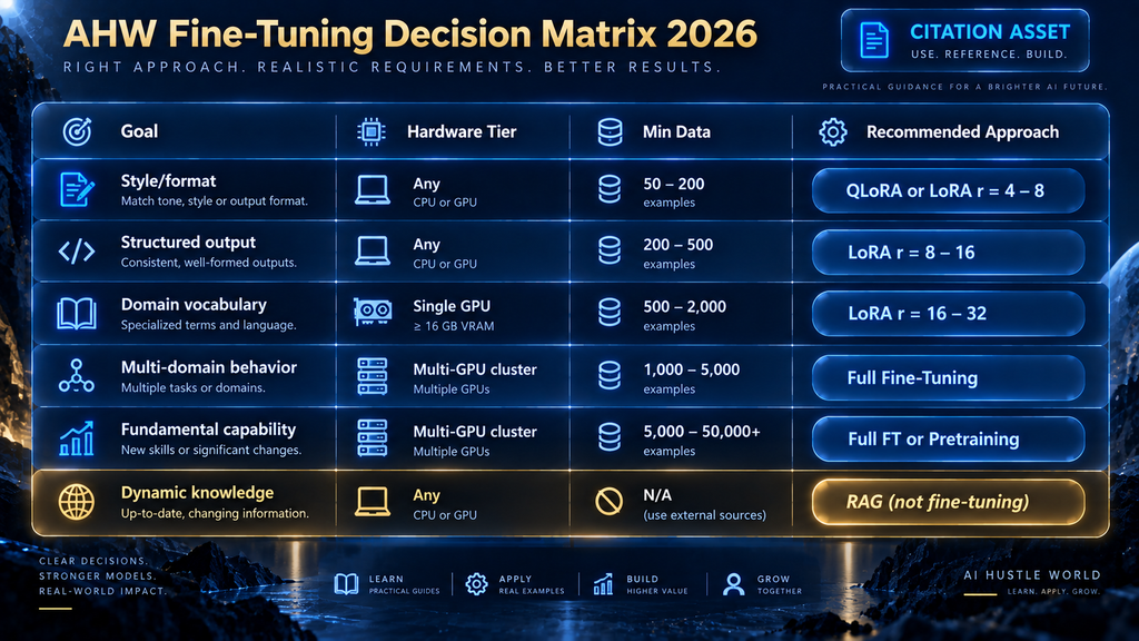
This framework maps your goal type, hardware tier, and minimum data needs to a recommended starting approach. It synthesizes VRAM guidance from Spheron (2026), dataset sizing from Particula.tech (2026), and practical escalation logic from Together AI into one reference.

Goal	Hardware Tier	Min Data Needed	Recommended Approach
Style/format consistency	Any	50–200 examples	QLoRA or LoRA (r=4–8)
Structured output (JSON, extraction)	Any	200–500 examples	LoRA (r=8–16)
Domain vocabulary adaptation	Single GPU ≥16 GB	500–2,000 examples	LoRA (r=16–32)
Multi-domain behavioral change	Multi-GPU cluster	1,000–5,000 examples	Full Fine-Tuning
Fundamental capability change	Multi-GPU cluster	5,000–50,000+ examples	Full Fine-Tuning or Pretraining
Dynamic knowledge / live data	Any	N/A	RAG (not fine-tuning)

Sources: Spheron 2026 VRAM analysis; Particula.tech 2026 dataset sizing guidance; Together AI fine-tuning recommendations. Framework synthesis and editorial structure: AI Hustle World.

Dataset Requirements: How Much Data You Actually Need

The answer everyone gives — “you need good quality data” — is technically true and practically useless without concrete numbers behind it. Here are the actual minimum thresholds by task type, based on Particula.tech’s 2026 analysis and validated against practical guidance from the Hugging Face fine-tuning documentation and Together AI.

Classification and routing tasks need 100–300 examples per category. If you’re training a model to route incoming customer queries, you need at least 100 clean, representative examples per routing category. Below that floor, few-shot prompting will almost certainly perform just as well — and the fine-tuning won’t generalize reliably to inputs that differ meaningfully from your training examples.

Structured output and extraction needs 200–500 examples. Teaching a model to consistently produce valid JSON with a specific schema, or to extract named fields from unstructured documents, requires enough variety in training examples to cover edge cases. The distribution of your inputs matters as much as the count — 200 examples that cover your actual input distribution will outperform 500 that only cover the easy cases.

Content generation and summarization needs 500–2,000 examples. Style transfer, tone adaptation, and constrained summarization require more data because the output space is far larger. The model needs to learn not just what you want in a specific format, but how to produce it naturally across a wide and varied range of inputs.

Complex domain adaptation (medical, legal, highly specialized technical) needs 1,000–5,000 examples. These domains have vocabulary, reasoning conventions, and output standards that diverge substantially from what the base model encountered during pretraining. The floor is higher because you’re not nudging style — you’re asking the model to develop specialized judgment on a domain where its defaults are genuinely weak.

The absolute floor across all task types is 50–100 examples. Below that, fine-tuning is almost always the wrong choice regardless of task type. At that data volume, few-shot prompting — discussed in depth in Few-Shot vs Zero-Shot Prompting — produces comparable or better results without the training cost or the risk of a poorly-generalized model.

The quality principle deserves equal weight to the quantity thresholds: 200 carefully curated, diverse, high-quality examples consistently outperform 2,000 mediocre ones. The most common fine-tuning failure isn’t data volume — it’s data quality. Duplicates, inconsistent formatting, examples that demonstrate the wrong behavior, and outputs that contradict each other all undermine training regardless of how many examples you have. Before generating more data, audit what you already have.

The Decision Framework: Which Approach to Use

The decision isn’t a binary choice between LoRA and full fine-tuning. It’s a three-step sequence, and each step filters the options before you get to the next one.

Step 1: Can prompt engineering or RAG solve this first?

If the behavior you want can be reliably triggered with a well-crafted system prompt and a few examples in context, fine-tuning is almost certainly the wrong tool. Prompt engineering is faster, cheaper, and fully reversible — you don’t need to re-train anything when requirements change.

RAG handles live knowledge without any training at all, which matters whenever the information you’re injecting changes frequently or varies by user. Context Engineering Explained covers how far the context window can actually take you before fine-tuning becomes necessary — and it’s further than most practitioners assume.

Reserve fine-tuning for use cases that genuinely require permanent behavioral change across every response — not just better responses when prompted correctly, but a consistent, structural difference in how the model behaves by default. Step 2: What are you trying to change, and what hardware do you have?

Consult the AHW Fine-Tuning Decision Matrix above. Map your specific goal to the recommended approach. The general rule: start with QLoRA if you have a consumer GPU or want low-cost iteration; use LoRA if you need higher-capacity adapters and have access to a 16–24 GB VRAM card; escalate to full fine-tuning only if you have multi-GPU infrastructure and have validated through earlier LoRA or QLoRA experiments that the task actually requires it.

Step 3: Do you have enough quality data for that approach?

Check your data volume against the thresholds in the dataset section above. If you’re below the minimum for your task type, invest in data preparation before training — not after a failed run. If you’re significantly above the minimum, the quality question is more important than the quantity question.

Together AI’s practical guidance is worth internalizing as a default posture: start with LoRA for efficiency and escalate to full fine-tuning only when performance plateaus and you’ve confirmed that the gap is meaningful for your actual application. The additional cost of full fine-tuning rarely justifies itself until you’ve proven through experimentation that LoRA can’t reach your quality target.

What the Research Actually Shows: LoRA vs Full Fine-Tuning

A widely-repeated assumption in the fine-tuning community is that LoRA and full fine-tuning produce essentially equivalent models — just through different training paths. A 2024 paper presented at NeurIPS challenges that assumption in ways that matter practically, particularly for anyone planning sequential or multi-task fine-tuning.

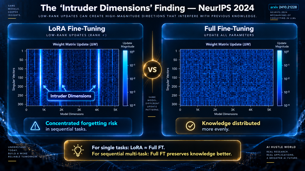
The paper (Biderman et al., 2024; arxiv 2410.21228) analyzed structural differences between LoRA-trained and fully fine-tuned models using singular value decomposition of the weight matrices. The finding: LoRA introduces what the researchers call “intruder dimensions” — new high-ranking singular vectors in the weight matrices that are entirely absent in models produced by full fine-tuning. These intruder dimensions are artifacts of the adapter’s low-rank structure being merged into the base model’s weights.

The practical implication is counterintuitive. In single-task fine-tuning, LoRA and full fine-tuning produce models that perform comparably — the intruder dimensions don’t cause meaningful problems when the model is doing one thing consistently and its task distribution is stable.

But in sequential multi-task fine-tuning — where you fine-tune the same model on Task A, then Task B, then Task C over time — LoRA models accumulate intruder dimensions across each fine-tuning pass and forget earlier tasks at higher rates than fully fine-tuned models. Forgetting doesn’t distribute evenly across the model’s knowledge. It concentrates specifically in those intruder dimensions, making the degradation harder to predict and mitigate.

For the majority of practitioners doing single-task fine-tuning on a stable use case, this finding changes nothing — LoRA remains the right default. But if your use case involves sequential fine-tuning across multiple domains, or updating a model over time as your task evolves across fine-tuning sessions, the research suggests full fine-tuning may preserve accumulated knowledge better in the long run, even at significantly higher cost. This nuance is almost universally absent from competing fine-tuning guides, and it’s worth understanding if your use case doesn’t fit the single-task mold.

When Fine-Tuning Fails: Catastrophic Forgetting, Overfitting and Alignment Regression

Fine-tuning can go wrong in three distinct ways, each with different causes and different remedies. Understanding them before you train is part of what separates practitioners who get reliable results from those who burn compute budget without understanding why the run failed.

Catastrophic forgetting happens when the model overwrites its general knowledge with the domain-specific patterns in your fine-tuning data. The result is a model that performs well on your specific task but fails badly on everything else — sometimes dramatically. A general reasoning question that the base model would handle confidently gets a confused or hallucinated response because the relevant parameters have been overwritten by your domain-specific training data.

The primary mitigations are Elastic Weight Consolidation (EWC) — a regularization technique that adds a penalty term to the loss function discouraging large changes to parameters that were important during pretraining — and rehearsal methods, which mix a small percentage of general-purpose data into the fine-tuning dataset so the model continues to see diverse inputs throughout training. LoRA’s approach of freezing base weights provides inherent protection against catastrophic forgetting for a single fine-tuning pass, which is one of the strongest practical arguments for preferring it over full fine-tuning when both would achieve comparable task quality.

Overfitting occurs when the model memorizes training examples rather than learning the underlying pattern. An overfitted model performs well on examples it was trained on and poorly on new inputs that differ in any meaningful way. The tell-tale signal is training loss that drops steadily while validation loss plateaus or starts rising — those two curves diverging is the diagnostic.

Early stopping — halting training when validation loss stops improving — is the most reliable remedy. Dropout regularization during training also helps, as does increasing the diversity of your training examples. If your validation and training curves diverge significantly, your dataset is almost certainly too small, too repetitive, or too narrowly scoped to support the generalization your application requires.

Alignment regression is the least-discussed but potentially most consequential failure mode. The safety and helpfulness properties instilled in an instruction-tuned model during its RLHF or DPO alignment process can be partially or fully undone by aggressive fine-tuning on a dataset that doesn’t reflect those properties. A model that was reliably helpful and safe to deploy can become evasive, inconsistent, or produce outputs that violate the behavioral constraints the base model had.

This risk is particularly significant when fine-tuning instruction-tuned or chat-optimized models rather than raw base models. The mitigation is deliberate: ensure your training data includes examples that demonstrate the behavioral norms you want to maintain — not just task examples — and explicitly evaluate the fine-tuned model’s safety and helpfulness properties before deploying it, not just its task performance. For context on how the underlying model architecture processes these behavioral norms, What Is a Large Language Model (LLM) and How AI Models Understand Language: Explained Simply for Beginners provide useful background.

Fine-Tuning vs Prompting vs RAG: Where Each Fits

These three approaches aren’t competitors in the sense that only one can be right — they address genuinely different problems, and in many production systems they’re used together.

Prompt engineering is the right starting point for nearly every use case, including ones that eventually need fine-tuning. It requires no training data, no compute cost, and is completely reversible when requirements change. Well-crafted prompts can handle style guidance, task instructions, output formatting, persona, and many types of behavioral constraints with surprising reliability.

The limitation is consistency at scale: everything you want the model to do has to fit into the context window, and the behavior can drift when prompts get long or when the instruction set grows complex enough to create internal tensions. Techniques like few-shot examples and chain-of-thought reasoning (covered in Few-Shot vs Zero-Shot Prompting) can push prompt engineering further than most practitioners initially expect.

RAG is the right tool when the information the model needs is dynamic, specific to the user or session, or too large to train on. Customer support systems that reference a constantly-updated knowledge base, research assistants that pull from live documents, and systems where relevant user-specific context varies widely across sessions are natural RAG use cases.

RAG keeps the model frozen — no training required, no alignment risk, no risk of overwriting existing knowledge — and the knowledge layer updates independently of the model. For a detailed treatment of how RAG works architecturally, The Complete Guide to Retrieval-Augmented Generation (RAG) covers the full stack. RAG’s limitation is that it can’t change how the model reasons or responds — only what information it has access to.

Fine-tuning is warranted when you need behavioral change that is consistent, deep, and can’t be reliably triggered through prompting alone. A model that consistently produces a specific output structure without being instructed to, a model that reasons with genuine competence in a specialized domain, or a model whose style and tone match a specific brand voice so consistently that no explicit persona prompt is needed — these are the cases fine-tuning earns its cost.

The practical decision flow: prompt engineering first, RAG if knowledge is dynamic and variable, fine-tuning if behavior needs to be permanent and consistent across every single response regardless of what the user provides.

An important practical note: many production systems use all three together. A fine-tuned model with a carefully engineered system prompt and a RAG layer for live knowledge retrieval is a common and highly effective architecture — particularly in customer-facing applications where both domain expertise (fine-tuning) and up-to-date information (RAG) matter simultaneously.

Final Thoughts

Fine-tuning has become accessible enough that practitioners who couldn’t have touched it three years ago — because it required expensive multi-GPU clusters and significant ML engineering infrastructure — can now run meaningful experiments on a single consumer GPU for a few dollars. QLoRA made that possible. LoRA made it scalable. The hardware cost barrier that once made fine-tuning a large-team exclusive is largely gone for model sizes up to 7B or 13B parameters.

What hasn’t changed is the requirement for clarity about what you’re trying to accomplish before you start training. The most common fine-tuning failure isn’t a technical error — it’s a wrong diagnosis. Practitioners fine-tune when prompt engineering would have worked. They reach for full fine-tuning when QLoRA would have sufficed. They under-invest in data quality and over-invest in compute. The AHW Fine-Tuning Decision Matrix in this article is designed specifically to short-circuit those mistakes by forcing the decision into a structured sequence before a single training step runs.

The right posture is to treat the escalation path — prompt engineering → RAG → QLoRA → LoRA → full fine-tuning — as a series of gates, not a spectrum to sample from freely. Each gate is cheaper, faster to validate, and easier to reverse than the one after it. You escalate when you’ve confirmed the previous approach can’t reach your quality target — not before. That discipline, more than any specific technical choice, is what separates practitioners who get reliable fine-tuning results from those who keep re-running expensive training jobs without understanding why they’re failing.

Frequently Asked Questions

What is the difference between fine-tuning and prompt engineering?

Prompt engineering gives the model instructions at inference time but doesn’t change its weights — the model’s underlying knowledge and behavior remain exactly the same across sessions. Fine-tuning updates the model’s parameters by continuing to train it on new data, producing lasting behavioral change that persists across every response without needing to repeat the instruction in every prompt. The practical distinction: if the behavior you want can be triggered consistently with a well-written prompt, prompt engineering is faster and cheaper. Fine-tuning becomes necessary when the behavioral change needs to be permanent, deep, and reliable without runtime instruction.

Do I need a GPU to fine-tune a language model?

For any model above about 1B parameters, yes — a GPU with sufficient VRAM is effectively required. That said, QLoRA has dramatically lowered the minimum hardware floor. A 7B model can be fine-tuned with QLoRA on a single RTX 4090 (24 GB VRAM), and cloud GPU providers like Modal, RunPod, and Lambda Labs offer access to sufficient hardware for $3–$10 per training run at that model size. For 70B models, even QLoRA still requires a high-end cloud GPU (approximately 52 GB VRAM), which means cloud compute rather than consumer hardware.

What is LoRA rank, and how do I choose it?

LoRA rank (r) controls how many parameters the adapters use and how expressive they can be. Low rank (r=4–8) is sufficient for style and formatting tasks. Medium rank (r=16–32) works well for domain vocabulary and structured output tasks. Higher rank (r=64+) is rarely necessary and significantly increases compute requirements. Start at r=8 and adjust based on validation loss — if the model isn’t converging, increase rank before assuming you need full fine-tuning.

How much training data do I need to fine-tune a model?

The minimum depends on task type. Classification tasks need 100–300 examples per category. Structured output and extraction tasks need 200–500 examples. Content generation and style tasks need 500–2,000 examples. Complex domain adaptation (medical, legal, highly specialized) needs 1,000–5,000 examples. Below 50–100 total examples, few-shot prompting is almost always the better choice. Data quality matters as much as quantity — 200 curated examples consistently outperform 2,000 mediocre ones.

What is catastrophic forgetting in fine-tuning?

Catastrophic forgetting is when a model overwrites its general knowledge with domain-specific training data, becoming specialized but losing broad competence. It’s most severe in full fine-tuning because all weights are updated simultaneously. Mitigations include Elastic Weight Consolidation (EWC), which penalizes large changes to parameters that were important during pretraining, and rehearsal methods that mix general-purpose examples into the fine-tuning dataset. LoRA provides inherent protection against catastrophic forgetting for single fine-tuning passes because the base weights stay frozen throughout training.

Is QLoRA as good as full fine-tuning?

For most single-task use cases, QLoRA quality is close enough to full fine-tuning that the quality gap doesn’t justify the cost difference — especially when you factor in the much faster iteration cycles. A 2024 NeurIPS paper (arxiv 2410.21228) found that LoRA and full fine-tuning produce structurally different models, with LoRA introducing “intruder dimensions” that can cause concentrated forgetting in sequential multi-task scenarios. For a single, well-defined task on a stable distribution, QLoRA is the right default. For sequential or multi-task fine-tuning over time, full fine-tuning may preserve knowledge better.

Can I fine-tune any AI model?

Not every model supports fine-tuning through every provider. Larger mixture-of-experts (MoE) models may be LoRA-only from certain providers due to architectural constraints. Proprietary hosted models depend on each provider’s fine-tuning offering, and those offerings change. OpenAI, for example, is winding down its self-serve fine-tuning platform: according to its deprecations page (checked 26 Sep 2026), organizations that had never run fine-tuning lost access on 7 May 2026, and from 6 Jan 2027 active customers can no longer create new fine-tuning jobs, although existing fine-tuned models keep running until their base model is retired. Open-weight models like Llama 3, Mistral, Qwen, and Gemma can be fine-tuned locally or on cloud compute with full flexibility over method, rank, and hyperparameters.

What is alignment regression and how do I avoid it?

Alignment regression is when fine-tuning partially undoes the safety and helpfulness properties that were instilled during a model’s instruction tuning or RLHF process. An instruction-tuned model that was reliable and safe to deploy can become evasive, inconsistent, or produce outputs that violate the behavioral boundaries the base model had. To avoid it: include examples in your training data that demonstrate the behavioral norms you want to maintain — not just task examples — and explicitly evaluate safety and helpfulness properties after fine-tuning, not just task performance. This is especially important when fine-tuning instruction-tuned or chat-optimized models rather than raw base models.

What is the difference between LoRA and full fine-tuning structurally?

In full fine-tuning, every weight in the model is updated during training. In LoRA, the base model weights are frozen and only the small adapter matrices (W_A and W_B) are trained, with their output added to the frozen base weights at inference time. This is why LoRA uses far less VRAM — you don’t need to store gradients and optimizer states for the full model, only for the adapters. It’s also why LoRA adapters are compact (often under 100 MB) while full fine-tuned models are the same size as the original model.

When should I use RAG instead of fine-tuning?

Use RAG when the information you need to inject is dynamic (changes frequently), user-specific (varies by session), or voluminous enough that training on it would be impractical. A frequently-updated company knowledge base, a live news feed, or a customer-specific document repository are all RAG use cases — not fine-tuning use cases. Fine-tuning is for behavioral change that should be consistent regardless of what external documents the model accesses. If what you need is the model to know more, RAG is almost always the better path. If what you need is the model to behave differently, fine-tuning is the right answer