How to Prepare a Dataset for Fine-Tuning a Language Model
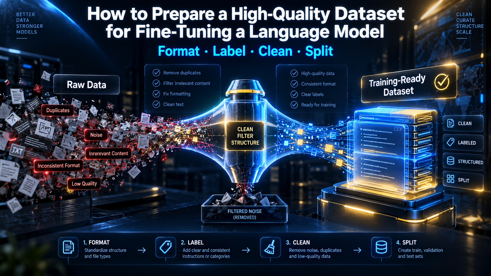
Most fine-tuning projects fail before the first training step. Not because of bad hyperparameters, wrong learning rates, or hardware constraints — but because the dataset going in was already broken. Bad labels, inconsistent formatting, leaked test data, length mismatches, or a thousand carefully curated examples that all say the same thing in slightly different ways. The model learns exactly what you give it. If you give it noise, it learns noise. If you give it a format that’s 80% consistent, it produces outputs that are 80% reliable — on a good day.
This guide is the one that most fine-tuning tutorials skip. They show you the training code. They show you transformers.Trainer. They show you what buttons to press in a notebook. But the dataset preparation — the actual work that determines whether you end up with a model that’s useful or a model that sounds confident while being wrong — gets maybe two paragraphs. Here, it gets the full treatment it deserves.
What this covers: Every stage of dataset preparation that materially affects fine-tuning quality — format selection, sizing, cleaning, deduplication, synthetic data, labeling quality, splitting, and tokenization. With the specific papers behind the claims, and the specific defects that show up as specific model failures when you get it wrong.
What this doesn’t cover: Model architecture choices, hyperparameter tuning, PEFT methods like LoRA (covered in our LoRA Explained guide), or inference optimization. This is purely about getting the dataset right before training starts.
The Quick Answer
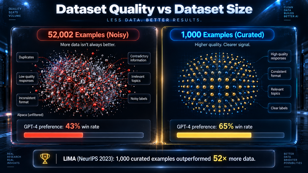
For most fine-tuning jobs, quality beats quantity by a wide margin. A curated dataset of 1,000 examples will consistently outperform 50,000 noisy examples — demonstrated repeatedly in peer-reviewed work. The most destructive defect is target-label noise (wrong answers in the “expected output” column). The most common mistake is treating data preparation as a preprocessing step when it’s actually the design work. And the five failure modes that reliably destroy fine-tuned models — rambling, hallucination, inflated evals, silent truncation, and over-refusal — are all data bugs in disguise.
Why Dataset Quality Beats Dataset Size
In 2023, Meta AI published a result that should have reset everyone’s expectations about fine-tuning data. The paper was called LIMA — Less Is More for Alignment. The team fine-tuned a 65B LLaMA model on exactly 1,000 carefully hand-selected examples covering diverse topics, tasks, and formats. No preference data. No reinforcement learning from human feedback. Just 1,000 examples. In human evaluation, LIMA was preferred over or tied with GPT-4 in 43% of comparisons, outperformed Alpaca in 58% of cases, and beat the text-davinci-003 model in 65% of direct comparisons. The paper is arXiv:2305.11206, published at NeurIPS 2023.
The AlpaGasus team pushed the same principle further. Starting from the 52,002-example Alpaca dataset, they used ChatGPT as a quality filter to score each instruction-response pair and kept only the top 9,229 examples. The filtered dataset produced models that matched or exceeded the full Alpaca baseline in the majority of benchmark comparisons, trained 5.7× faster, and at 13B parameters, achieved over 90% of GPT-4’s performance on quality-scored outputs. That paper is arXiv:2307.08701, published at ICLR 2024.
The mechanism behind both results is the same. When you add low-quality examples to a training set, you’re not just adding neutral noise — you’re actively degrading the signal. The model has to average across your good examples and your bad ones. Every mislabeled, inconsistently formatted, or duplicate example pulls the learned weights slightly in the wrong direction. And because these effects compound across thousands of gradient steps, what starts as minor data sloppiness ends as major model unreliability.
This doesn’t mean you can fine-tune on 50 examples and expect miracles. It means you should spend the time you’d otherwise put into finding more data and put it into making your existing data better. That tradeoff almost always pays off.
What Fine-Tuning Actually Learns — and What It Doesn’t
Before you can make good dataset decisions, you need an accurate mental model of what fine-tuning actually changes in a language model. The intuition most people have — that you’re adding knowledge to the model by training on domain-specific data — is wrong, and it leads to bad data choices.
Arnav Gudibande and colleagues at UC Berkeley ran a direct test of this in 2023. They fine-tuned models on outputs from stronger teacher models (GPT-4, Claude) and then evaluated whether the student models had actually learned the factual knowledge those outputs contained. The answer was no. The student models learned to sound like the teacher — matching response style, tone, structure, and hedging patterns — but their factual accuracy on knowledge-intensive tasks didn’t improve. The paper, “The False Promise of Imitating Proprietary LLMs,” describes this as learning surface form without acquiring the underlying capability.
A 2024 ICML paper by Ghosh et al. (arXiv:2402.05119) went further, testing whether instruction-tuning adds knowledge that wasn’t already in the base model. It doesn’t. Their benchmark showed that instruction tuning primarily teaches format and response behavior — how to structure outputs, when to decline, how to handle multi-step requests. The knowledge was already baked in during pretraining. To demonstrate the practical implication: in their experiments, LoRA fine-tuning on just 1,000 LIMA examples outperformed standard SFT on datasets 52× and 326× larger when evaluated on factuality.
What this means for your dataset: if you’re trying to teach the model facts, you’re using the wrong tool. Fine-tuning teaches behavior. If you want a model that knows your product catalog, knows your company’s policies, or can answer questions about your proprietary documentation — build a RAG pipeline instead. Save fine-tuning for what it’s actually good at: teaching the model how to respond, not what to know.
For more on how fine-tuning fits into this broader picture, see our introduction to fine-tuning language models.
The Five Red Flags: When Bad Data Shows Up as Bad Model
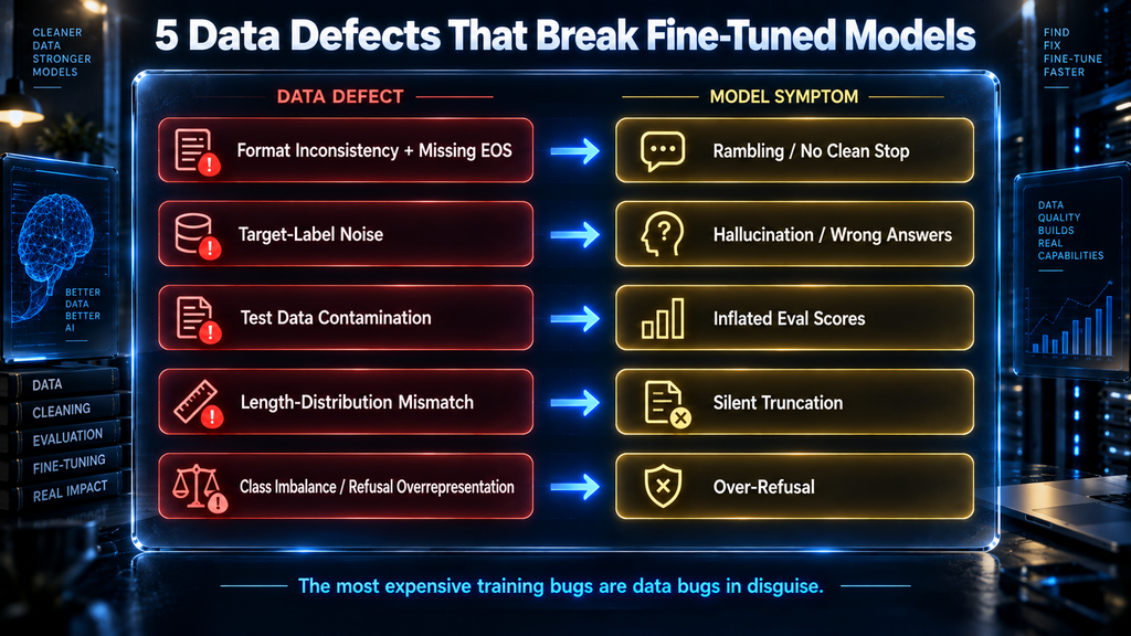
Every dataset defect has a downstream failure mode. The link between cause and effect isn’t always obvious — you train your model, it misbehaves, and you assume the learning rate was wrong. It usually wasn’t. Here are the five defects that matter most, and what each one produces.
1. Format inconsistency and missing EOS tokens → rambling outputs. When training examples use inconsistent system prompt structure, switch between capitalization conventions, or omit end-of-sequence tokens, the model never learns a clean stopping signal. The result is a model that continues generating after the answer is complete, adds unnecessary caveats, repeats itself, or fails to terminate properly. If your model ramps on endlessly, check your format before you check your temperature.
2. Target-label noise → hallucination and degraded factuality. This is the most destructive defect in supervised fine-tuning datasets, and it’s well-documented in the research literature. A 2025 label noise study (arXiv:2604.12469) confirmed that noise on the target side — wrong expected outputs — is significantly more damaging than input-side noise. The model learns to confidently produce the wrong answer. Unlike random output errors, which are visible, label noise teaches systematic errors that pattern-match plausibly to real outputs. Spotting it in a deployed model is hard. Spotting it in your data before training is much easier.
3. Data contamination and test leakage → inflated evaluations that measure nothing. If examples from your evaluation benchmarks appear in your training set — either directly or through paraphrasing — your evaluation scores become meaningless. A 2024 NAACL paper by Deng et al. found contamination rates of 29.1% in MMLU and 45.8% in C-Eval across commonly used open models. These aren’t edge cases. They’re systematic problems in widely deployed models that were trained on scraped internet data without contamination checks. For custom fine-tuning, the same risk exists whenever your evaluation set is drawn from the same source as your training set.
4. Length-distribution mismatch → silent truncation. Every tokenizer has a context window. If your training data is dominated by short examples but your deployment inputs are long — or vice versa — you have a distribution mismatch the model can’t compensate for. More concretely: if your target responses are longer than the model’s max sequence length during training, they get silently truncated. The model trains on incomplete examples. The completion is cut off mid-sentence, with no signal that anything is wrong. You don’t know this is happening unless you plot the sequence length distribution of your dataset before training. It’s a ten-minute analysis that prevents weeks of mysterious model failures.
5. Class imbalance and refusal overrepresentation → over-refusal. If your training set contains significantly more refusal responses than action responses — or significantly more of any one response type — the model overfits toward that type. The most common version of this is a model that refuses reasonable requests because refusals were overrepresented in the safety or alignment data. Measure class distribution before training. Rebalance if the ratio is more than roughly 3:1 for any critical category.
Data Formats: Alpaca, ShareGPT, Completion, and Preference
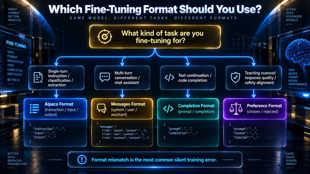
Getting the format right is not optional. It’s the load-bearing structure of your training pipeline. The format determines how the model learns to interpret roles, when to speak and when to listen, what constitutes a complete response, and how it handles multi-turn context. Choose the wrong format for your task and you’ll spend weeks troubleshooting problems that are actually format mismatches.
Alpaca Format
The Alpaca format is flat JSON with three fields: instruction, input, and output. It was introduced with the original Alpaca dataset in 2023 and is still widely used for single-turn instruction fine-tuning.
The input field is optional — for tasks that don’t require additional context, it’s left empty. Alpaca format is the right choice for single-turn tasks with a clear instruction-to-output pattern: classification, summarization, entity extraction, translation, and similar. It’s not suited for multi-turn conversations.
ShareGPT / Messages Format
The messages format (also called ShareGPT format after the dataset that popularized it) uses an array of role-labeled turns: system, user, and assistant. This is the format native to most modern chat models and the right choice for conversational fine-tuning, multi-turn dialogue, and any task where context builds across exchanges.
If you’re fine-tuning for a chat assistant, an agent, or any use case where the model needs to maintain context across a conversation, use this format. It’s also what most instruction-following models (LLaMA 3, Mistral, Qwen) are pre-trained with, so it’s the most natural extension of what the base model already knows.
Completion / Prompt-Completion Format
The simplest format. A prompt field and a completion field. No roles, no system messages. This format is best for continuation tasks — code generation where you’re providing a function signature and expecting an implementation, text continuation, or any task where the model is extending rather than responding.
Preference Formats (DPO, ORPO, SimPO)
Preference formats — used for Direct Preference Optimization and related methods — require pairs of responses labeled as chosen and rejected. They’re used to teach the model relative quality distinctions rather than absolute right/wrong outputs.
The chosen response demonstrates the quality behavior you want; the rejected response demonstrates what you’re training away from. Preference data requires significantly more annotation effort than standard SFT data, but it’s the right tool when you need to teach nuanced quality distinctions — better tone, more appropriate explanation depth, safer handling of edge cases — that can’t be captured by a single “correct” answer.
Dataset Sizing: The Evidence-Backed Curve
One of the most common questions in fine-tuning is “how many examples do I need?” The honest answer is that it depends heavily on the task. But the research gives us concrete benchmarks to work from, and a clear pattern: diminishing returns set in earlier than most people expect.
Data-to-Task Sizing Table
| Task Type | Recommended Example Range | Notes | Key Source |
|---|---|---|---|
| Classification (2–5 classes) | 200–500 | Returns plateau quickly with balanced classes | Standard SFT baselines |
| Classification (10+ classes) | 500–2,000 | More classes require proportionally more examples per class | — |
| Single-turn instruction following | 500–2,000 | LIMA shows 1,000 curated examples sufficient for broad alignment | LIMA, NeurIPS 2023 |
| Domain-specific Q&A | 500–1,500 | Quality dominates quantity; AlpaGasus shows 9,229 beats 52,002 | AlpaGasus, ICLR 2024 |
| Multi-turn dialogue / chat | 1,000–5,000 | Needs diverse turn structures and lengths | — |
| Code generation (narrow domain) | 300–1,000 | Models have strong pretraining priors; less fine-tuning needed | — |
| Code generation (broad) | 1,000–5,000 | Depends on language and task diversity | — |
| Enterprise task specialization | 200–600 | Research shows plateau past ~600 examples for narrow tasks | arXiv:2503.01870 |
| Summarization | 500–2,000 | Length variation in training set matters significantly | — |
| Preference/alignment data (DPO) | 1,000–10,000 | Fewer, higher-quality chosen/rejected pairs beat noisy large sets | — |
These are starting points, not ceilings. If your task is broad, your domain is unusually specialized, or your quality bar is high, you’ll need more. But these numbers reflect where the research shows meaningful gains — and where adding more data without improving quality stops paying off.
The enterprise plateau finding (arXiv:2503.01870) is particularly useful for narrow-task fine-tuning. For highly specific enterprise use cases — a customer service bot for a single product line, a classifier for a narrow document type — performance often plateaus around 600 examples. Beyond that, adding more similar examples produces negligible improvement while increasing training cost and the risk of overfitting.
For overfitting prevention strategies when working with small datasets, see our upcoming guide on preventing overfitting in fine-tuned models.
Data Cleaning: The Work Nobody Advertises
The least glamorous part of dataset preparation is also the part that produces the most reliable improvement. Cleaning removes what’s actively damaging your training signal.
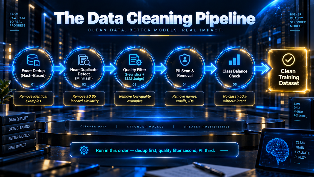
Exact Deduplication
Exact duplicates — two identical training examples — teach the model to weight that pattern more heavily than any other, because the same gradient is applied multiple times. In large datasets scraped from the internet, duplicate rates of 10–30% are common. Lee et al. (arXiv:2107.06499) showed that exact-substring deduplication and MinHash near-duplicate removal both improve perplexity and downstream task performance, with exact deduplication being the faster and more straightforward first pass.
For small to medium datasets (under 100,000 examples), a hash-based exact deduplication is fast and sufficient as a first pass. Sort your training JSONL by text hash, find collisions, drop them. This takes minutes and removes some of the most damaging examples in your dataset.
Near-Duplicate Detection
Near-duplicates are more expensive to find but often more important to remove. A dataset scraped from a content farm or generated from a single template might contain thousands of examples that differ by only a few words. The model learns the shared structure excessively — at the cost of learning anything else.
MinHash with Locality Sensitive Hashing (LSH) is the standard approach for datasets above 10,000 examples. You define a similarity threshold (commonly 0.8–0.9 Jaccard similarity) and remove one example from each near-duplicate pair. SimHash offers a faster alternative for very large datasets. For most fine-tuning datasets in the 1,000–50,000 range, MinHash with an 0.85 threshold is sufficient and can be implemented in Python with the datasketch library in under 50 lines.
Filtering for Quality
Deduplication removes redundancy. Quality filtering removes the bad examples that remain after deduplication. The two main approaches are heuristic filtering and LLM-as-judge filtering.
Heuristic filtering applies rules to remove examples that are likely low quality: minimum and maximum length thresholds, punctuation ratio checks, language detection (to remove mixed-language noise), and format validation (is the JSONL actually parseable? does it have all required fields?). These rules are cheap to apply and catch a large fraction of obvious problems.
LLM-as-judge filtering — prompting a capable model to score each training example on quality dimensions — is more expensive but more accurate. AlpaGasus used this approach to filter 52,002 Alpaca examples down to 9,229, using ChatGPT to rate each example on a 1–5 scale and keeping only examples rated 4 or 5. The resulting dataset outperformed the original despite being less than 18% of the original size.
The practical trade-off: use heuristics first to remove the obvious garbage cheaply, then apply LLM-as-judge to the remainder if your dataset is large enough to make further filtering valuable.
PII Removal
Any dataset that contains personally identifiable information — real names, email addresses, phone numbers, physical addresses, account numbers, or in some jurisdictions, IP addresses — must have that information removed or masked before training. A model trained on PII can reproduce it in outputs, which creates both legal exposure and user trust problems.
Standard approaches: regex-pattern removal for structured PII (emails, phone numbers, SSNs), named entity recognition for less structured PII (person names in context), and scrubbing tools like Microsoft Presidio or the anonymizers library for systematic detection. For datasets likely to contain medical or financial PII, manual review of a random sample after automated scrubbing is worth doing. Automated tools have false negative rates that matter at scale.
Class Balance
Measure the distribution of your training labels or response types before training. If you’re doing classification, is each class represented roughly proportionally? If you’re doing instruction fine-tuning, what percentage of your examples are refusals, factual Q&A, creative writing, code, and conversational responses?
Significant imbalance (one class comprising more than 50–60% of examples for a multi-class task, or one response type dominating a general-purpose dataset) will bias the model toward that class or type in proportion to the imbalance. The fix is either augmenting underrepresented classes, downsampling overrepresented ones, or applying class weighting in the loss function — the right choice depends on whether you have enough data in the underrepresented class to make augmentation meaningful.
Synthetic Data: What It Can and Can’t Do
Generating synthetic training data with a capable model — GPT-4, Claude, Gemini — is now standard practice. It’s fast, cheap, and scalable. But it comes with structural limitations that are important to understand before committing to a synthetic data strategy.
The foundational synthetic data approach is Self-Instruct, introduced by Wang et al. in 2022 (arXiv:2212.10560, ACL 2023). Start with a small seed set of human-written examples, use a language model to generate new instructions and completions, filter for quality and diversity, repeat. The original paper generated 82,000 instruction-response pairs from 175 seed tasks using GPT-3, producing a model (InstructGPT) that matched text-davinci-001 on crowdworker evaluations. The approach works. At scale, with a capable generator model, you can produce large, diverse, formatted datasets cheaply.
What synthetic data teaches well: response format and structure, the distribution of a particular response style, task-completion patterns for well-defined tasks (extraction, classification, translation), and conversational behavior patterns. If you want a model that responds in a specific format or tone, synthetic data from a model that already demonstrates that format or tone is an efficient way to capture it.
What synthetic data doesn’t teach: factual knowledge the base model doesn’t already have, factual accuracy beyond the generator model’s own accuracy, or any capability that requires grounding in real-world data the generator can’t access. This is the same finding as Gudibande et al. — synthetic data, like imitation data, transfers style and format, not knowledge or factual reliability.
The deeper risk is model collapse. Shumailov et al. published a study in Nature (2024, DOI: 10.1038/s41586-024-07566-y) demonstrating that iterative training on model-generated data — where each generation’s outputs become the next generation’s training data — causes progressive degradation in output diversity and quality. The distribution narrows, tails collapse, and the model becomes less capable of generating anything that diverges from the central tendency of its training distribution. They called this “model collapse,” and it’s a real risk for any pipeline that recursively generates synthetic data without consistently mixing in human-curated examples.
The practical rule: synthetic data is a useful tool for augmenting a human-curated seed dataset, not a replacement for it. Mix synthetic and human-verified data. Never train solely on the outputs of a previous version of your own model without reintroducing human-verified ground truth.
Labeling Quality: The Human Work That Makes or Breaks Everything
For datasets with human-generated labels or human-written responses, annotation quality is where most of the value is created — and most of it is destroyed. Two researchers reading the same piece of text and applying the same labeling rubric will frequently disagree. The question is how much they disagree, how to measure it, and how to reduce it.
Inter-Annotator Agreement
Inter-annotator agreement (IAA) measures how consistently multiple annotators apply the same labels to the same examples. The standard metrics:
Cohen’s κ (kappa) — for two annotators on a categorical task. Adjusts for chance agreement. Values above 0.8 indicate strong agreement; 0.6–0.8 is moderate; below 0.6 is poor. If your two annotators have Cohen’s κ below 0.7 on your main labeling dimension, your rubric is underspecified and needs revision before you continue annotating.
Fleiss’ κ — the generalization to three or more annotators on categorical tasks. Same interpretation scale as Cohen’s κ.
Krippendorff’s α — more general, handles ordinal, interval, and ratio scales in addition to categorical. Preferred when your labels have ordering (quality ratings on a 1–5 scale) or when annotators occasionally skip items.
Measure IAA at the start of every annotation project, before generating the bulk of your data. A small calibration set — 50–100 examples with multiple annotators — will reveal whether your rubric is producing consistent results or whether you need to add more examples, more specificity, or explicit decision trees for common edge cases.
The Ceiling Effect
A common labeling trap: your rubric is defined at the task level, not the edge case level. Annotators agree perfectly on the easy examples and diverge significantly on the 15–20% of examples that require judgment. Since the easy examples dominate the dataset, your overall IAA looks fine while the examples that most need reliable labels have high disagreement.
The fix is to analyze IAA specifically on the disagreement examples — the subset where any two annotators chose different labels. If that subset has low IAA, your rubric needs additional guidance precisely for those cases. Adding labeled edge-case examples to the annotator guidelines (not just rules, but real instances with explanations of the correct label and why) typically reduces disagreement more than rewriting the rules in the abstract.
Common Labeling Errors
Anchoring on the first example. Annotators who see a high-quality example first will calibrate their quality scale relative to it, making subsequent moderate examples seem worse than they are. Randomize presentation order and provide calibration examples that span the full quality range.
Leniency and severity bias. Some annotators systematically assign higher scores; others systematically assign lower ones. This introduces systematic error even when annotators appear to agree on relative rankings. If you’re using quality ratings, recalibrate annotator baselines after the initial calibration batch.
Fatigue degradation. Annotation accuracy degrades over long sessions. If you’re labeling more than 300–400 examples per annotator per session on a judgment-intensive task, expect measurable quality decline in the later batches. Schedule shorter annotation sessions and mix in recalibration examples throughout.
The AHW Dataset Readiness Checklist
Before any fine-tuning run, a complete dataset review should happen at the format, quality, splitting, and hygiene levels. This checklist covers the minimum required before training.
Format Gate
- All examples use a single consistent format (Alpaca, messages, completion, or preference — not mixed)
- Every example has all required fields and no unexpected fields
- EOS tokens are present at the end of every completion
- System prompt is identical (or intentionally varied) across all examples — not inconsistently duplicated or missing
- JSONL parses without error (validate with
python -c "import json; [json.loads(l) for l in open('data.jsonl')]") - Role labels are consistent (
user/assistantnot mixed withhuman/botor other variants) - No null or empty fields in required positions
Quality Gate
- Quality filter applied (heuristic or LLM-as-judge) — low-quality examples removed
- Label accuracy validated on a random sample (minimum 100 examples reviewed)
- No systematic bias in completions (not dominated by a single response pattern or template)
- Instruction-response pairs are genuinely paired (instructions match their completions)
- No obvious placeholder text or generation artifacts (
[INSERT HERE],As an AI language model...openings, etc.)
Splitting Gate
- Train / validation / test split defined before any other processing
- Stratified split applied if class imbalance exists
- Test set is fully held out — no examples from it appear in training data
- Evaluation benchmark examples checked against training data for contamination
Hygiene Gate
- Exact deduplication complete (hash-based)
- Near-duplicate check complete (MinHash or SimHash, threshold ≥ 0.85)
- PII scan complete — no names, emails, phone numbers, addresses in training examples
- Language distribution confirmed (no unintended multilingual contamination)
- Sequence length distribution plotted — no silent truncation of target completions
- Class/category distribution measured — no category exceeds 50% without intent
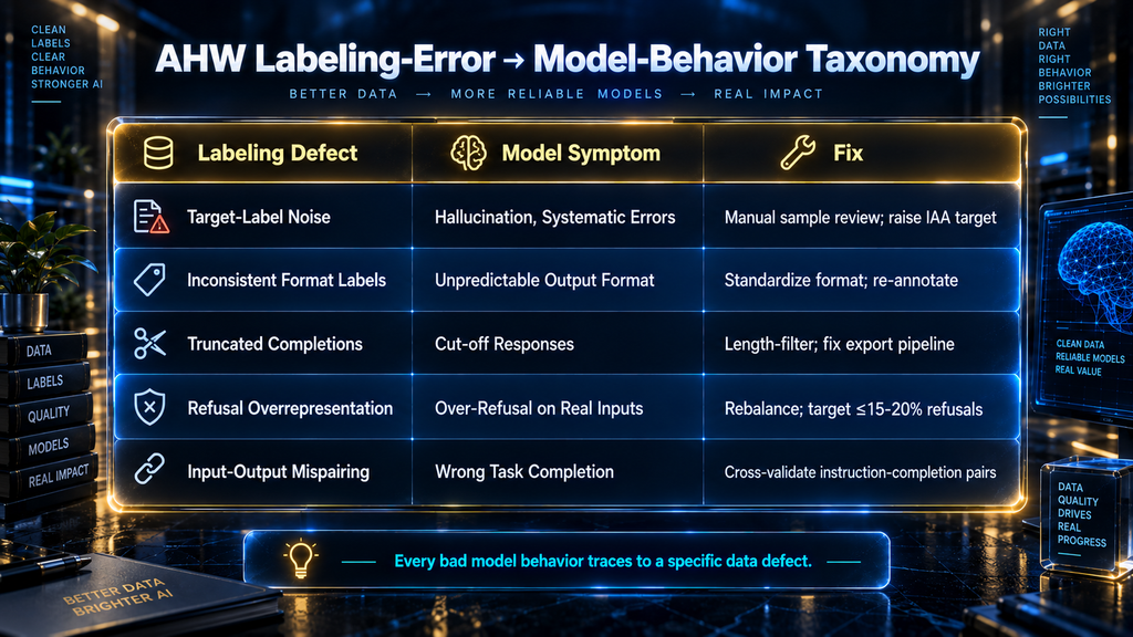
The Labeling-Error → Model-Behavior Taxonomy
The link between a specific labeling defect and a specific model behavior is not always intuitive. This taxonomy maps the five most common labeling defects to the model symptoms they produce and the remediation approach.
| Labeling Defect | What It Looks Like in Data | Model Symptom | Remediation |
|---|---|---|---|
| Target-label noise (wrong expected output) | Completion says “Paris” when the answer is “Berlin”; summarization extracts wrong claim | Hallucination, systematic factual errors that pattern-match to common mistakes | Manual review of random completion sample; remove or correct mislabeled examples; measure IAA before scaling annotation |
| Inconsistent format labeling | Some examples use JSON output; others use plain text; role labels differ | Model produces inconsistent output format; switches between formats unpredictably | Standardize format across all examples; re-annotate the inconsistent subset; enforce format with explicit system prompt |
| Incomplete completions (truncated labels) | Completion is cut off mid-sentence due to length filtering or export error | Model produces cut-off or abrupt responses; fails to complete complex instructions | Plot completion length distribution; remove examples below minimum meaningful completion length; validate exports |
| Refusal / “I can’t do that” overrepresentation | 40%+ of training examples are refusals across a dataset meant for task performance | Over-refusal on legitimate inputs; model declines reasonable requests citing safety | Rebalance by adding positive examples; measure class distribution; target ≤15–20% refusal rate for task-oriented fine-tuning |
| Input-output mispairing | Instruction is “Translate to Spanish” but completion is in French; summary doesn’t match provided text | Incorrect task completion; model seems to “misunderstand” even clear instructions | Cross-validate instruction-completion pairs; automated checks where the relationship can be verified programmatically (language detection, semantic similarity) |
Train, Validation, and Test Splits
The split is not a detail. It’s the structure that determines whether your evaluation means anything.
The standard split for fine-tuning datasets is 80/10/10 — 80% training, 10% validation, 10% test. For datasets smaller than 1,000 examples, consider an 85/15 train/validation split with a separately curated test set drawn from a different source than the training data. The validation set is what you use during training to monitor for overfitting and tune hyperparameters. The test set is touched exactly once — after training is complete — to produce the final reported evaluation metrics.
Always create your splits before any other processing. This is a common ordering mistake: people deduplicate, filter, and clean the full dataset and then split. If near-duplicate pairs end up on both sides of a split, your model trains on something semantically identical to what it’s being evaluated on. The deduplication should happen within the training set, not across the split boundary, and the split should be created first.
For classification and other tasks with meaningful class labels, use stratified splitting — ensuring that each class is represented proportionally in each split. A simple random split on a dataset with significant class imbalance will frequently produce a test set that’s missing rare classes entirely.
Protecting the test set from contamination means exactly one thing in practice: no one looks at the test set until the final evaluation, and nothing from the test set is used to make any decision about the model — not cleaning decisions, not hyperparameter choices, not architecture decisions. The moment you use test set performance to guide any upstream decision, it’s no longer a test set. It’s a validation set, and you need a new test set.
Tokenization and Packing
The final step before training is tokenization, and it introduces two decisions that significantly affect training efficiency and model behavior.
Sequence Length Distribution
Before tokenizing, plot the distribution of your training examples after tokenization. For each example, count the total tokens (prompt + completion for chat formats, or the full sequence for completion formats). You need to answer three questions:
- What percentage of examples exceed your max sequence length? Any example that’s longer than the model’s context window during training will be truncated. If that truncation cuts through the completion — the part you’re actually trying to train — you’re training on incomplete examples with no signal that they’re incomplete.
- What’s the average and median sequence length? If the vast majority of your examples are 50–100 tokens but your context window is 4,096, you’re wasting significant computation on padding.
- Are there outliers? A small number of very long examples can disproportionately affect training dynamics if you’re not aware of them.
Padding vs. Packing
The two strategies for handling variable-length examples in batches: padding and packing.
Padding adds special pad tokens to the end of shorter examples to make all examples in a batch the same length. It’s simple, clean, and safe — but wastes computation on tokens that don’t contribute to learning. At short average sequence lengths with large context windows, padding waste can reach 50% (arXiv:2107.02027).
Packing concatenates multiple short examples into a single sequence, separated by EOS tokens, filling the context window more efficiently. The efficiency gain is real: a 2025 ACL Findings paper (arXiv:2410.08081) showed that packing matches or beats padding on downstream task performance across models up to 34B parameters, with the advantage growing at larger model sizes.
The risk with packing is cross-contamination: if the model can attend across the boundary between two packed examples, it may learn spurious associations between them. This is mitigated by proper attention masking — ensuring that attention from one packed example cannot attend to tokens in a different packed example in the same sequence. Frameworks like Hugging Face TRL’s DataCollatorForCompletionOnlyLM handle this correctly. If you implement packing yourself, verify the attention masks.
Common Dataset Preparation Mistakes
Skipping the length distribution plot. The single most common preventable mistake. Takes five minutes to produce and catches silent truncation, excessive padding waste, and outlier examples that will crash your training loop.
Using the full dataset for deduplication before splitting. Near-duplicate pairs that end up on both sides of your train/test split make your evaluation metrics meaningless. Always split first, then deduplicate within splits.
Confusing instruction diversity with example diversity. Having 2,000 examples that ask the same underlying question in slightly different words is not a diverse dataset. Diversity means covering different task types, different domains, different difficulty levels, different output structures. Measure diversity explicitly — the QDIT diversity framework (arXiv:2311.14736) showed that maximizing instruction-following diversity improved worst-case benchmark robustness by 18%.
Treating synthetic data as equivalent to human-verified data. It isn’t. Use synthetic data to augment a human-curated core, not to replace it. A 1,000-example human-curated seed with 4,000 synthetic augmentations is significantly more reliable than 5,000 synthetic examples generated without human review.
Annotating before aligning the rubric. Writing annotation guidelines and immediately handing them to annotators without a calibration run leads to systematic disagreement that compounds across thousands of examples. Run a 50–100 example calibration batch, measure IAA, revise the rubric where annotators diverge, and repeat until Cohen’s κ is above 0.7 before scaling.
Adding more data instead of fixing the existing data. When a fine-tuned model performs poorly, the instinct is to gather more training examples. Usually, you should review a random sample of 100 existing examples first. In a significant fraction of cases, you’ll find the problem — label noise, format inconsistency, truncation — before you’ve collected a single new example.
Final Thoughts: Your Data Bugs Are Disguised as Model Bugs
There’s a persistent assumption in the fine-tuning community that model problems are model problems. A model that hallucinates needs better training or a different architecture. A model that over-refuses needs better RLHF. A model that generates in the wrong format needs better prompting.
Frequently, these are dataset problems. The hallucination traces back to mislabeled completions that taught the model to be confidently wrong. The over-refusal traces back to a training set where 40% of the examples were refusals. The format inconsistency traces back to a dataset that mixed Alpaca and messages format without anyone noticing.
The research on this is consistent. Fine-tuning teaches behavior, not knowledge. Label noise on the target side is the most destructive defect. Synthetic data transfers style and not facts. Dataset size past the diminishing-returns threshold buys you nothing. What the data teaches is what the model does.
The most experienced practitioners in this field — the people who’ve built production fine-tuned models that work reliably — spend more time on data than on everything else combined. Not because training is easy. But because they’ve learned that the training runs which fail were decided long before the training loop started.
Build the dataset with the same care you’d give to the architecture. Because for fine-tuning purposes, the dataset is the architecture. Every decision about what goes in, what gets cleaned out, how it’s labeled, and how it’s split is a decision about what your model will do. Make those decisions deliberately, and make them first.
Your Dataset Is Ready. Now Choose the Right Training Method.
Most fine-tuning jobs don’t need full-weight training — they need LoRA. Understand how Low-Rank Adaptation works, how to pick the right rank, and why it outperforms full fine-tuning on most real-world datasets before you run your first training loop.
Read: LoRA Explained →Frequently Asked Questions
How many examples do I need to fine-tune a language model?
For a narrow, well-defined task, 500–1,000 high-quality examples is a practical starting point. LIMA showed 1,000 curated examples can rival much larger models. Enterprise task specialization often plateaus around 600 examples. Quality matters far more than quantity — a curated 1,000 beats a noisy 50,000 in controlled studies.
What’s the difference between SFT and preference fine-tuning?
Supervised fine-tuning (SFT) trains the model to produce a single “correct” output given an input. Preference fine-tuning (DPO, ORPO, SimPO) trains the model on pairs of outputs — one preferred, one rejected — and teaches relative quality distinctions. SFT is faster and simpler; preference fine-tuning is better for teaching nuanced response quality.
Can I use GPT-4 generated data to fine-tune a smaller model?
Yes — and Self-Instruct, AlpaGasus, and many other approaches do exactly this. It’s effective for transferring format and response style. The important caveat: the student model learns to sound like the teacher but doesn’t inherit the teacher’s factual knowledge or accuracy. For factual tasks, combine synthetic data with human verification.
What is data contamination and why does it matter?
Data contamination is when examples from your evaluation benchmarks appear in your training data. It makes benchmark results meaningless — the model has “seen” the answers. Research found 29.1% contamination in MMLU and 45.8% in C-Eval across widely used models. Always check your training data against your evaluation benchmarks before training.
Should I use Alpaca format or the messages format?
Use messages format for any conversational or multi-turn use case. Use Alpaca format for simple single-turn instruction tasks (classification, extraction, translation). Most modern models are pre-trained in messages format, so it’s the more natural fit for most fine-tuning scenarios.
What causes a fine-tuned model to ramble or not stop?
Usually missing or inconsistent EOS tokens in the training data. The model never learned a clean stopping signal. Check that every completion in your training set ends with the tokenizer’s EOS token, and that you’re using consistent formatting throughout.
How do I detect label noise in my training data?
Review a random sample of at least 100 examples manually — specifically checking that the completion is factually correct, relevant to the instruction, and doesn’t contradict the instruction’s intent. For classification datasets, compute inter-annotator agreement on a sample. Label noise above 5–10% on the target side will meaningfully degrade model quality.
Is synthetic data safe to use for fine-tuning?
Yes, with constraints. Synthetic data is effective for format, style, and task-pattern transfer. It’s not effective for teaching factual knowledge. Don’t train recursively on model-generated data without mixing in human-curated examples — iterative training on purely synthetic data causes model collapse (demonstrated in Nature, 2024). Use synthetic data to augment human-curated seeds, not to replace them.
How should I split my dataset for fine-tuning?
Standard is 80/10/10 (train/validation/test). Always create the split before cleaning or deduplication — not after. Use stratified splitting if your data has class labels. Hold out the test set completely and evaluate on it only once, after all training decisions are final.
What’s the biggest mistake people make in fine-tuning dataset preparation?
Skipping the audit before training. Most practitioners run data prep and immediately train. Spending 30–60 minutes reviewing a random sample of 100 examples — checking label accuracy, format consistency, completion length, and class distribution — catches the majority of problems that would otherwise only surface after an expensive training run.
Related Guides
- What Is a Large Language Model (LLM)? How LLMs Really Work
- What Is an AI Agent? A Beginner’s Guide to How Autonomous AI Works
- How to Use AI Tools Safely: A Complete Learning Path
Written by
Muntasir Ahmad Chowdhury
Founder, AI Hustle World
Muntasir Ahmad Chowdhury is the Founder of AI Hustle World, an independent publication dedicated to making Artificial Intelligence practical, trustworthy, and easy to understand. He researches AI tools, automation, customer service, productivity, and real-world business applications, helping readers make smarter technology decisions through research-driven, experience-backed content.
Expertise:
AI Tools • AI Automation • AI Customer Service • AI Productivity • Generative AI • AI Workflows
Get Smarter With AI
Enjoyed this guide? Get practical AI tools, tutorials, and honest reviews delivered to your inbox.
4 thoughts on “How to Prepare a Dataset for Fine-Tuning a Language Model”